Bayesian dynamic forecasting
Dynamic forecasting is a common prediction tool after fitting multivariate time-series models, such as vector autoregressive (VAR) models. It predicts outcome values at a current time by using updated (predicted) outcome values at previous times. The new bayesfcastcommand computes Bayesian dynamic forecasts after fitting a Bayesian VAR model by using the bayes: var command.
Bayesian dynamic forecasts produce an entire sample of predicted outcome values at each time point instead of a single prediction as in classical analysis. This sample can be used to answer various modeling questions, such as how well the model predicts future observations without making the asymptotic normality assumption when estimating forecast uncertainty. This is particularly appealing for small datasets for which the asymptotic normality assumption may be suspect.
You can use bayesfcast compute to compute dynamic forecasts and save them in the current dataset, and you can graph them by using bayesfcast graph.
Let’s see it work
We continue with the U.S. macrodata from Bayesian VAR models, which are quarterly data from the first quarter of 1954 to the fourth quarter of 2010. We would like to obtain Bayesian dynamic forecasts of inflation, output gap, and federal funds rate from a Bayesian VAR model for these variables.
Here is what the data look like.
. webuse usmacro
(Federal Reserve Economic Data - St. Louis Fed)

. tsset

Time variable: date, 1954q3 to 2010q4
        Delta: 1 quarter

. tsline inflation ogap fedfunds

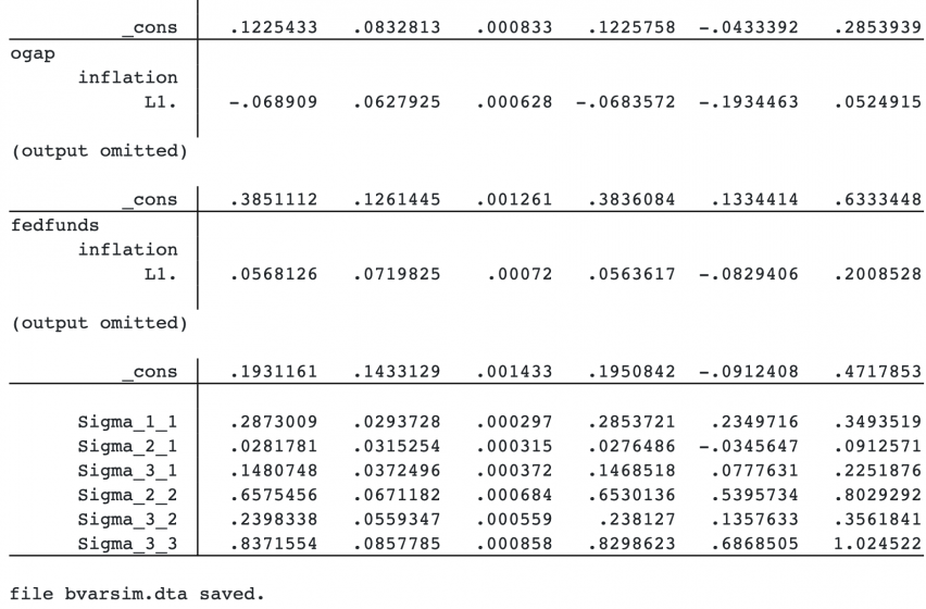
We first fit a Bayesian VAR model with four lags. To check our forecast performance, we will hold our data after the first quarter of 2004. We also save MCMC results in bvarsim.dta.
The output from the bayes: var command is long, so we omit some of it below.
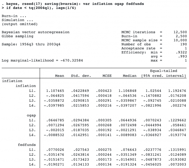
See Bayesian VAR model for details about bayes: var and its output.
We use the new bayesfcast command to compute Bayesian dynamic forecasts. This command has two subcommands. bayesfcast compute computes the forecasts and saves them in the current dataset as new variables. And bayesfcast graph plots the forecasts.
Let’s start with the simplest specification. We specify f_ as the prefix for the new variables and a random-number seed for reproducibility.
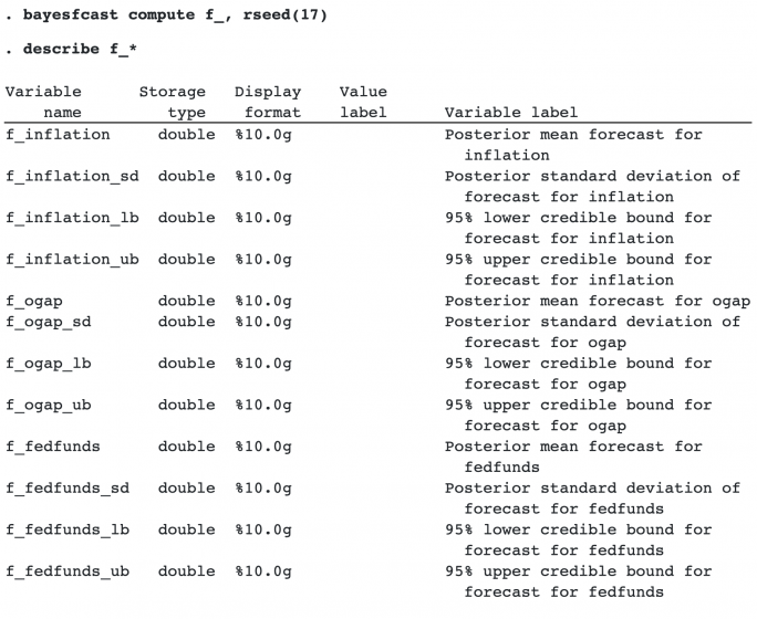
bayesirf compute creates new variables containing various summary statistics for forecasts. Unlike with classical analysis, a Bayesian forecast at a specific time corresponds to not just one value but a sample of MCMC values. These values are then summarized (as means or medians) to provide a single statistic. By default, the command computes posterior means, posterior standard deviations, and 95% equal-tailed credible intervals for the forecast for each outcome variable.
Let’s plot the default forecasts and their 95% equal-tailed credible bands.
. bayesfcast graph f_inflation f_ogap f_fedfunds

By default, we obtain one-period forecasts. We later show how to create forecasts with more periods.
Instead of posterior mean forecasts and equal-tailed credible intervals, we can compute posterior median forecasts and highest posterior density (HPD) credible intervals. We compute and plot them below.
. bayesfcast compute f_, rseed(17) median hpd replace
. bayesfcast graph f_inflation f_ogap f_fedfunds

If we want to explore trends in forecasts, we need more time periods. For instance, below we specify 28 periods in the step() option of bayesfcast compute.
. bayesfcast compute f_, step(28) rseed(17) replace
. bayesfcast graph f_inflation f_ogap f_fedfunds, observed
We compare our forecasts with the observed values. The forecasts appear to do well in predicting outcomes up until 2007. After that, they perform poorly. For instance, the 95% credible intervals for the output gap do not contain the observed values for part of the time horizon.

After the analysis, we remove the MCMC simulation file saved by bayes: var.
. erase bvarsim.dta