Multivariate meta-analysis

Univariate meta-analysis deals with a single effect reported by each study. However, there are many cases in practice where a study may report multiple effect sizes. For example, does the keto diet, the high-protein diet, the vegan diet, or intermittent fasting achieve the highest amount of weight loss? Each of these comparisons will generate an effect size. Modeling each effect separately ignores the fact that they may be correlated. Multivariate meta-analysis models the effects jointly and accounts for their dependence.

Let’s see it work

Multivariate meta-analysis

Example dataset: Treatment of moderate periodontal disease

Constant-only model: Multivariate meta-analysis

Incorporating moderators: Multivariate meta-regression

Random-effects estimation methods and between-study covariance structure

estat heterogeneity

Postestimation: Predicting random effects

Multivariate meta-analysis

Suppose we are interested in investigating the effect of multiple dietary regimens on weight loss. Multiple effect sizes that compare each of these diets with a control group (not following any diet) can be computed. These effect sizes are usually correlated because they share a common control group. Or perhaps we want to explore the impact of a new teaching technique on math (outcome 1), physics (outcome 2), and chemistry (outcome 3) testing scores. Three effect sizes that compare the three testing scores across two groups of students (those who were taught using the new technique and those who were not) are computed. These three effect sizes are dependent because they were calculated using the same set of students.

Example dataset: Treatment of moderate periodontal disease

Consider a dataset from Antczak-Bouckoms et al. (1993) of five randomized controlled trials that explored the impact of two (surgical and nonsurgical) procedures on treating periodontal disease. Two outcomes of interest are improvements from baseline (pretreatment) in probing depth (y1) and attachment level (y2) around the teeth. The main objectives of the periodontal treatment were to reduce probing depths and increase attachment levels (Berkey et al. 1998). Because the two outcomes y1 and y2 are measured on the same subject, they should not be treated as independent.

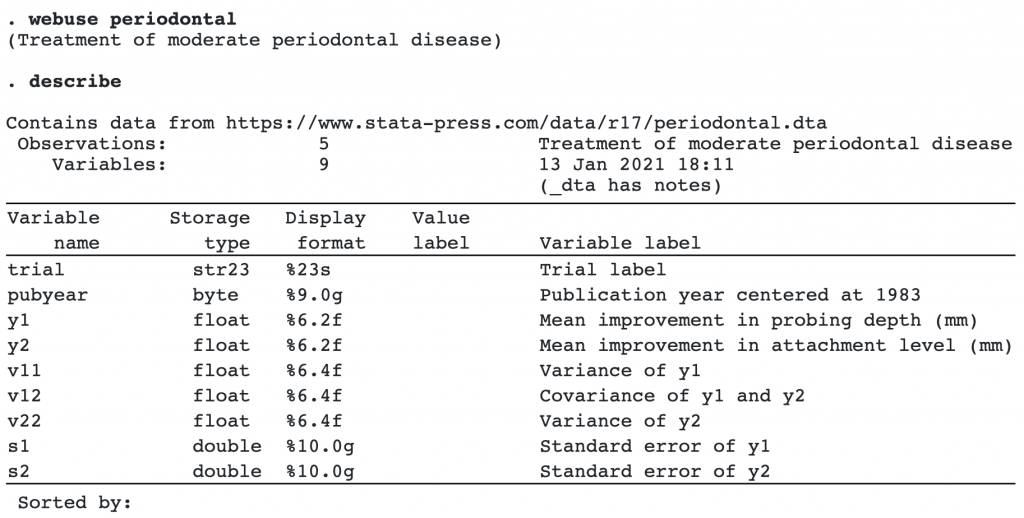
Variables v11, v12, and v22 define the within-study covariance matrix for each study.

Constant-only model: Multivariate meta-analysis

If we were to perform two separate univariate meta-analyses for outcomes y1 and y2, we would be ignoring the dependence among the two outcomes, which may lead to incorrect inference. We use the command meta mvregress to conduct a bivariate meta-analysis as follows:

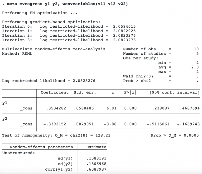
The order in which you specify variables within wcovvariables() is important (see wcovvariables() in [META] meta mvregress for details).

The first table displays the regression (fixed-effects) coefficient estimates from the bivariate meta-analysis. These estimates correspond to the overall bivariate effect sizes. The overall improvement in probing depth is roughly 0.35 mm, and the overall attachment level was reduced by 0.34 mm.

The multivariate homogeneity test, which tests whether the bivariate effect sizes (θ1j,θ2j) are constant across studies, is rejected (p < 0.0001).

The second table displays the standard deviations of the random effects corresponding to outcomes y1 and y2, as well as their correlation.

We could have performed a fixed-effects multivariate meta-analysis by specifying option fixed:

. meta mvregress y1 y2, wcovvariables(v11 v12 v22) fixed
(output omitted)

By performing a fixed-effects multivariate meta-analysis, we assume that study-specific bivariate effect sizes are the same across the studies and that the observed variability is due to sampling error. This assumption is often not satisfied in practice.

Incorporating moderators: Multivariate meta-regression

Berkey et al. (1998) argued that as the surgical experience accumulates, the surgical procedure will become more efficient, so the most recent studies may show greater surgical benefits. We will include variable pubyear, a surrogate for the time when the trial was performed, as a moderator to explain a portion of the heterogeneity highlighted in the previous section.

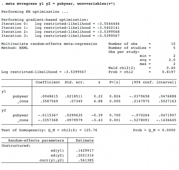
In the wcovvariables() option, we used the stub notation v* to refer to variables v11, v12, and v22.

The estimates of the regression coefficients of variable pubyear are 0.0049 with a 95% CI of [−0.0380, 0.0477] for outcome y1 and −0.0115 with a 95% CI of [−0.0703, 0.0472] for outcome y2. The coefficients are not significant according to the z tests, with the respective p-values, p = 0.824 and p = 0.7. It appears that pubyear did not explain the heterogeneity among the effect sizes.

Random-effects estimation methods and between-study covariance structure

Here we modify the default REML estimation method and use the ML estimation instead. We also use an independent covariance structure for the random effects. This may be done by specifying random(mle, covariance(independent)).

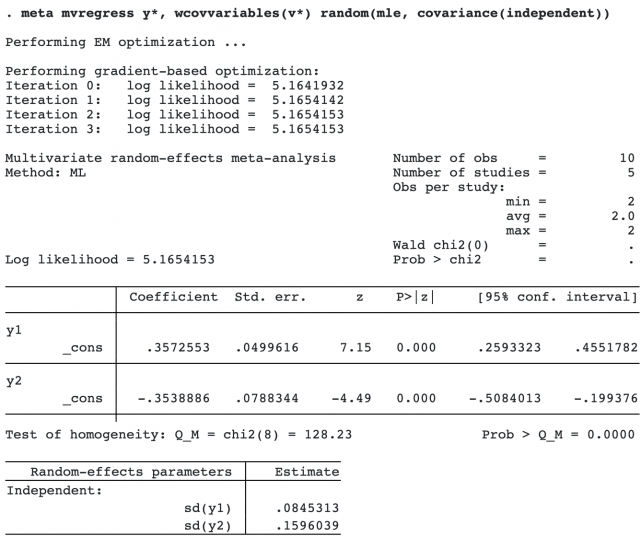
The random-effects parameter table now reports two terms, sd(y1) and sd(y2), because the correlation is assumed to be 0 under the independent covariance structure assumption.

estat heterogeneity

After you fit your multivariate meta-analysis model, you should quantify the amount of heterogeneity among the studies that was not accounted for by the model. You can use estat heterogeneity to do that.

. estat heterogeneity


Method: Cochran
Joint:
  I2 (%) = 93.76
      H2 = 16.03

Method: Jackson–White–Riley
y1:
  I2 (%) = 67.29
       R =  1.75

y2:
  I2 (%) = 94.40
       R =  4.23

Joint:
  I2 (%) = 87.49
       R =  2.83

This command produces heterogeneity statistics that extend the concept of univariate heterogeneity statistics, such as Q and I2, to the multivariate setting.

For instance, Cochran’s I2= 93.76% means that 93.76% of the heterogeneity is due to true heterogeneity between the studies as opposed to the sampling variability.

One potential shortcoming of the Cochran statistics is that they quantify the amount of heterogeneity jointly for all outcomes. The Jackson–White–Riley statistics provide ways to assess the contribution of each outcome to the total heterogeneity, in addition to their joint contribution.

For example, we can see that there is more heterogeneity among the effect sizes of outcome y2 (I2= 94.40%) than among the effect sizes of y1 (I2= 67.29%)

Postestimation: Predicting random effects

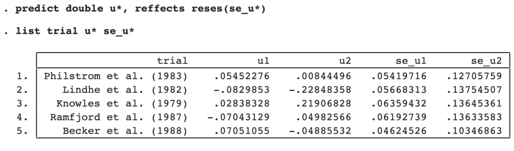
We listed the random-effects variables u1 and u2 with their corresponding standard-error variables se_u1 and se_u2. The random effects are study-specific deviations from the overall mean effect size. For example, for study 1 and outcome y1, the predicted mean improvement in probing depth is about 0.05 mm higher than the overall mean improvement in probing depth, θ̂ 1= 0.357.