Heckman selection models adjust for bias when some outcomes are missing not at random. Imagine modeling income. The problem is that income is observed only for those who work. Missingness is not random.

 

Stata fits Heckman selection models and, new in Stata 16, Stata can fit them with panel (two-level) data.

 

You want to fit the model

 

yit=xitβ+αi+εityit=xitβ+αi+εit

 

where yityit is sometimes missing. The equation that determines which yityit are not missing is

 

yit=zitγ+vi+uit>0yit=zitγ+vi+uit>0

 

In these equations, αiαi, εitεit, vivi, and uituit will not be estimated. Their correlations with each other, however, will be estimated along with ββ and γγ.

 

The above model can be fit even though income is not observed for everyone and even if their employment status changes over time.

 

Why fit a selection model? Because it is possible that people who work and whose income is therefore observed systematically differ from those who do not, and those differences are for unobserved reasons.

 

For instance, if more productive people work, their income will be higher than those who do not work. Or, if income of the less productive is lower, they might need to work more. Allowing for selection allows for either of the above alternatives and other alternatives too. After estimation, we can test whether selection matters.

 

Let’s see it work

 

We have fictional data on 8,000 individuals from 2011 to 2018. Among the variables are income, which is observed only for those who work. We worry that unobservables might lead to biased results.

 

To fit the selection model, we must model income and the probability of working. We model probability of working as a function of experience, age, region of the county, and whether the person has college or technical college training.

 

We fit the model

 

. xtheckman income c.age##c.age i.training#(c.exp##c.exp), select(working = age exp i.region i.training)

 

If you are new to Stata, things like c.age##c.age mean to include age and age squared in the model. The “c.” means continuous. The “i.” in i.training and i.region means categorical variable and indicates the categories are to be included in the model.

The results are

 

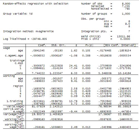
The first panel in the results reports the income equation.

 

The second panel reports the working (selection) equation.

 

After that are reported three variances and two correlations. The correlations are of interest.

 

correlation	estimate	SE
corr(e.working. e.income)	-0.58	0.06
corr(working[id], income[id])	0.26	0.10

 

The first correlation is the correlation of the residuals in the income and working (selection) equation, the correlation of εitεit and uituit.

 

The second is the correlation of random effects and unobservables that do not change over time, or the correlation of αiαi and vivi.

 

Selection was an issue if either of these correlations are significant. Both are.