GOALS 

This tutorial builds on the previous Linear Regression and Generating Residuals tutorials. It is suggested that you complete those tutorials prior to starting this one.

This tutorial demonstrates how to test the OLS assumption of error term normality. After completing this tutorial, you should be able to:

• Estimate the model using ols and store the results.
• Plot a histogram plot of residuals.
• Graph a standardized normal probability plot (P-P plot).
• Plot the quantiles of residuals against the normal distribution quantiles (Q-Q Plot).

INTRODUCTION 

In previous tutorials, we examined the use of OLS to estimate model parameters. One of the assumptions of the OLS model is that the error terms follow the normal distribution. This tutorial is designed to test the validity of that assumption.

In this tutorial we will examine the residuals for normality using three visualizations:

• A histogram of the residuals.
• A P-P plot.
• Q-Q plot.

ESTIMATE THE MODEL AND STORE RESULTS 

As with previous tutorials, we use the linear data generated from

where ϵi is the random disturbance term.

This time we will stored the results from the GAUSS function ols for use in testing normality. The ols function has a total of 11 outputs. The variables are listed below along with the names we will assign to them:

• variable names = nam
• moment matrix x’x = m
• parameter estimates = b
• standardized coefficients = stb
• variance-covariance matrix = vc
• standard errors of estimates = std
• standard deviation of residuals = sig
• correlation matrix of variables = cx
• r-squared = rsq
• residuals = resid
• durbin-watson statistic = dw

 // Clear the work space
 new;

// Set seed to replicate results
 rndseed 23423;

// Number of observations
 num_obs = 100;

// Generate independent variables
 x = rndn(num_obs, 1);

// Generate error terms
 error_term = rndn(num_obs,1);

// Generate y from x and errorTerm
 y = 1.3 + 5.7*x + error_term;

// Turn on residuals computation
 _olsres = 1;

// Estimate model and store results in variables
 screen off;
 { nam, m, b, stb, vc, std, sig, cx, rsq, resid, dbw } = ols("", y, x);
 screen on;

print "Parameter Estimates:";
 print b';

The above code will produce the following output:

Parameter Estimates:
       1.2795490        5.7218389

CREATE A HISTOGRAM PLOT OF RESIDUALS 

Our first diagnostic review of the residuals will be a histogram plot. Examining a histogram of the residuals allows us to check for visible evidence of deviation from the normal distribution. To generate the percentile histogram plot we use the plotHistP command. plotHistP takes the following inputs:

• myPlot
  • Optional input, a plotControl structure
• x
  • Mx1 vector of data.
• v
  • Nx1 vector, breakpoints to be used to compute frequencies or scalar, the number of categories (bins).

// Set format of graph
 // Declare plotControl structure
 struct plotControl myPlot;

// Fill 'myPlot' with default histogram settings
 myplot = plotGetDefaults("hist");

// Add title to graph
 plotSetTitle(&myPlot, "Residuals Histogram", "Arial", 16);

// Plot histogram of residuals
 plotHistP(myPlot, resid, 50);

The above code should produce a plot that looks similar to the one below. As is expected, these residuals show a tendency to clump around zero with a bell shape curve indicative of a normal distribution.

CREATE A STANDARDIZED NORMAL PROBABILITY PLOT (P-P)

As we wish to confirm the normality of the error terms, we would like to know how this distribution compares to the normal density. A standardized normal probability (P-P) can be used to help determine how closely the residuals and the normal distribution agree. It is most sensitive to non-normality in the middle range of data. The (P-P) plot charts the standardized ordered residuals against the empirical probability  , where i is the position of the data value in the ordered list and N is the number of observations.

There are four steps to constructing the P-P plot:

• Sort the residuals
• Calculate the cumulative probabilities from the normal distribution associated with each standardized residual   
• Construct the vector of empirical probabilities  
• Plot the cumulative probabilities on the vertical axis against the empirical probabilities on the horizontal axis

SORT THE RESIDUALS

GAUSS includes a built-in sorting function, sortc. We will use this function to sort the residuals and store them in a new vector, resid_sorted. sortc takes two inputs:

• x
  • Matrix or vector to sort.
• c
  • Scalar, the column on which to sort.

 //Sort the residuals
 resid_sorted = sortc(resid, 1);

Note: When sortc is used to sort a matrix, it does not return a matrix in which all columns are in ascending order. Instead, it sorts a specified column in ascending order and rearranges the other columns so that the rows stay together.

CALCULATE THE P-VALUE OF STANDARDIZED RESIDUALS

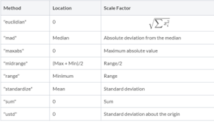
We need to find the cumulative normal probability associated with the standardized residuals using the cdfN function. However, we must first standardize the sorted residuals by subtracting their mean and dividing by the standard deviation, . This is accomplished using GAUSS’s data normalizing function, rescale. With this function, data can be quickly normalized using either pre-built methods or user-specified location and scaling factor. The available scaling methods are:

// Standardize residuals
 { resid_standard, loc, factor} = rescale(resid_sorted,"standardize");

// Find cummulative density for standardized residuals
 p_resid = cdfn(resid_standard);

Tip: When evaluating competing models, it is sometimes preferred to use the same location and scale parameters to scale the test or validation set as were used to scale the training set. For this reason, rescale will return the location and scale parameters when a named scaling method is used.

CONSTRUCT A VECTOR OF EMPIRICAL PROBABILITIES

We next find the empirical probabilities, , where $i$ is the position of the data value in the ordered list and  is the number of observations.

 // Calculate p_i
 // Count number of residuals
 N = rows(resid_sorted);

// Construct sequential vector of i values 1, 2, 3...
 i = seqa(1, 1, N);

// Divided each element in i by (N+1) to get vector of p_i
 p_i_fast = i/(N + 1);
 print p_i_fast;

Tip: We could have used a for loop to generate the empirical probabilities. However, it is most computationally efficient to use matrix operations in place of loops. For this reason we use the vector i rather than looping through single values of i.

© 2024 Aptech Systems, Inc. All rights reserved.

PLOT THE CUMULATIVE PROBABILITIES ON THE VERTICAL AXIS AGAINST THE EMPIRICAL PROBABILITIES

Our final step is to generate a scatter plot of the sorted residuals against the empirical probabilities. Our plot shows a relatively straight line, again supporting the assumption of error term normality.

/*
** Plot sorted residuals vs. corresponding z-score
*/
// Declare 'myPlotPP' to be a plotControl structure
// and fill with default scatter settings
struct plotControl myPlotPP;
myPlotPP = plotGetDefaults("scatter");
// Set up text interpreter
plotSetTextInterpreter(&myPlotPP, "latex", "axes");
// Add title to graph
plotSetTitle(&myPlotPP, "Standardized P-P Plot", "Arial", 18);
// Add axis labels to graph
plotSetYLabel(&myPlotPP, "NormalF\\ [ \\frac{x-\\hat{\\mu}}{\\hat{\\sigma}}\\ ]", "Arial", 14);
plotSetXLabel(&myPlotPP, "\\ p_{i}");
plotScatter(myPlotPP, p_i_fast, p_resid);

CREATE A NORMAL QUANTILE-QUANTILE (Q-Q) PLOT

A normal quantile-quantile plot charts the quantiles of an observed sample against the quantiles from a theoretical normal distribution. The more linear the plot, the more closely the sample distribution matches the normal distribution. To construct the normal Q-Q plot we follow three steps:

• Arrange residuals in ascending order.
• Find the Z-scores corresponding to N+1 quantiles of the normal distribution, where N is the number of residuals.
• Plot the sorted residuals on the vertical axis and the corresponding z-score on the horizontal axis

ARRANGE RESIDUALS IN ASCENDING ORDER

Because we did this above we can use the already created variable, resid_sorted.

FIND THE Z-SCORES CORRESPONDING THE N+1 QUANTILES OF THE NORMAL DISTRIBUTION, WHERE N IS THE NUMBER OF RESIDUALS.

To find Z-scores we will again use the cdfni function. We first need to find the probability levels that correspond to the n+1 quantiles. This can be done using the seqa function. To determine what size our quantiles should be, we divide 100% by the number of residuals.

 // Find quantiles
 quant_increment = 100/(n+1);
 start_point = quant_increment;
 quantiles=seqa(start_point, quant_increment, n);

// Find Z-scores
 z_values_QQ = cdfni(quantiles/100);

PLOT SORTED RESIDUAL VS. QUANTILE Z-SCORES

The Q-Q plot charts the sorted residuals on the vertical axis against the quantile z-scores on the horizontal axis. Where the P-P plot is good for observing deviations from the normal distribution in the middle, the Q-Q plot is better for observing deviations from the normal distribution in the tails.

 /*
 ** Plot sorted residuals vs. corresponding z-score
 */

// Declare plotControl struct and fill with default scatter settings
 struct plotControl myPlotQQ;
 myPlotQQ = plotGetDefaults("scatter");

// Set up text interpreter
 plotSetTextInterpreter(&myPlotQQ, "latex", "all");

// Add title to graph
 plotSetTitle(&myPlotQQ, "Normal\\ Q-Q\\ Plot","Arial", 16);

// Add axis label to graph
 plotSetXLabel(&myPlotQQ, "N(0,1)\\ Theoretical\\ Quantiles");
 plotSetYLabel(&myPlotQQ, "Residuals", "Arial", 14);

// Open new graph tab so we do not
 // overwrite our last plot
 plotOpenWindow();

// Draw graph
 plotScatter(myPlotQQ, z_values_QQ, resid_sorted);

CONCLUSION

Congratulations! You have:

• Stored results from the ols procedure.
• Created a histogram plot of residuals.
• Created a P-P graph of the residuals.
• Created a Q-Q graph of the residuals.

The next tutorial examines methods for testing the assumption of homoscedasticity.

For convenience, the full program text is reproduced below.

// Clear the work space
new;
// Set seed to replicate results
rndseed 23423;
// Number of observations
num_obs = 100;
// Generate independent variables
x = rndn(num_obs, 1);
// Generate error terms
error_term = rndn(num_obs,1);
// Generate y from x and errorTerm
y = 1.3 + 5.7*x + error_term;
// Turn on residuals computation
_olsres = 1;
// Estimate model and store results in variables
screen off;
{ nam, m, b, stb, vc, std, sig, cx, rsq, resid, dbw } = ols("", y, x);
screen on;
print "Parameter Estimates:";
print b';
// Declare plotControl structure
struct plotControl myPlot;
//Fill 'myPlot' with default histogram settings
myplot = plotGetDefaults("hist");
// Add title to graph
plotSetTitle(&myPlot, "Residuals Histogram", "Arial", 16);
// Plot histogram of residuals
plotHistP(myPlot, resid, 50);
// Sort the residuals
resid_sorted = sortc(resid, 1);
// Standardize residuals
{ resid_standard, loc, factor} = rescale(resid_sorted,"standardize");
// Find cummulative density for standardized residuals
p_resid = cdfn(resid_standard);
// Calculate p_i
// Count number of residuals
N = rows(resid_sorted);
// Construct sequential vector of i values 1, 2, 3...
i = seqa(1, 1, N);
// Divided each element in i by (N+1) to get vector of p_i
p_i_fast = i/(N + 1);
print p_i_fast;
/*
** Plot sorted residuals vs. corresponding z-score
*/
// Declare 'myPlotPP' to be a plotControl structure
// and fill with default scatter settings
struct plotControl myPlotPP;
myPlotPP = plotGetDefaults("scatter");
// Set up text interpreter
plotSetTextInterpreter(&myPlotPP, "latex", "axes");
// Add title to graph
plotSetTitle(&myPlotPP, "Standardized P-P Plot", "Arial", 18);
// Add axis labels to graph
plotSetYLabel(&myPlotPP, "NormalF\\ [ \\frac{x-\\hat{\\mu}}{\\hat{\\sigma}}\\ ]", "Arial", 14);
plotSetXLabel(&myPlotPP, "\\ p_{i}");
plotScatter(myPlotPP, p_i_fast, p_resid);
// Find quantiles
quant_increment = 100/(n+1);
start_point = quant_increment;
quantiles=seqa(start_point, quant_increment, n);
// Find Z-scores
z_values_QQ = cdfni(quantiles/100);
/*
** Plot sorted residuals vs. corresponding z-score
*/
// Declare plotControl struct and fill with default scatter settings
struct plotControl myPlotQQ;
myPlotQQ = plotGetDefaults("scatter");
// Set up text interpreter
plotSetTextInterpreter(&myPlotQQ, "latex", "all");
// Add title to graph
plotSetTitle(&myPlotQQ, "Normal\\ Q-Q\\ Plot","Arial", 16);
// Add axis label to graph
plotSetXLabel(&myPlotQQ, "N(0,1)\\ Theoretical\\ Quantiles");
plotSetYLabel(&myPlotQQ, "Residuals", "Arial", 14);
// Open new graph tab so we do not
// overwrite our last plot
plotOpenWindow();
// Draw graph
plotScatter(myPlotQQ, z_values_QQ, resid_sorted);