We are interested in the effect of an unexpected increase in interest rates (fedfunds) on industrial production growth (ip_growth) and inflation (inflation). We are concerned that the interest rate is endogenous: changes in interest rates affect other economic variables, but the interest rate itself responds to those same economic variables. We need to account for this potential endogeneity to reliably estimate the effects of the shock to interest rates. An instrumental-variables approach allows us to do this. We have an instrument, money_inst, that isolates exogenous changes to the interest rate. We can use the new ivlpirf command to estimate structural IRFs for the effects of an interest rate increase on industrial production growth response, using money_inst as an instrument for the endogenous impulse change in interest rate (d.fedfunds):
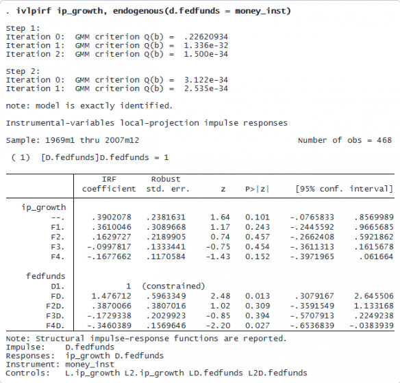
The output table displays IRF coefficients for the effect on impact (labeled –.) and for four periods after impact (labeled F1. through F4.). With an IRF coefficient of 0.39, we see a positive effect of an interest rate change on instustrial production growth on impact, but we do not have evidence that the effect is different from zero. It might take time for the effects of an interest rate change to be seen in industrial production, so longer horizons could be necessary to view the effect. The interest rate response is normalized to 1 on impact. The interest rate enters the model measured in changes (D.fedfunds), so subsequent coefficients on fedfunds are also changes. The change in interest rate rises by 1 percentage point on impact by construction, then changes in the same direction by 1.48 percentage points in the subsequent period, and so on.
The estimates above display IRFs that are expressed in the units of the variables—in this case, growth rates. We might also be interested in the cumulative response, which can be interpreted as the change in the level of the variable and can be calculated by summing the responses of the growth rates. ivlpirf supports this calculation with the cumulative option. Below, we specify ivlpirf with the cumulative option to report cumulative IRFs. We also compute the effects on two response variables (ip_growth and inflation) simultaneously.
© Copyright 1996–2026 StataCorp LLC. All rights reserved.
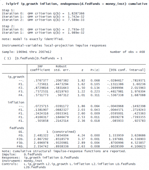
The coefficient table now displays the cumulative IRFs. They can be interpreted as the responses of industrial production (not industrial production growth), of price (not price inflation), and of interest rate (not change in interest rate) to the shock.
Rather than estimating only the default 4 months of responses, let’s use the step() option to estimate 3 years (36 months) of responses. Instead of looking at all of these cumulative IRFs in output table from ivlpirf, we will graph them using the irf commands.
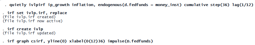
In the fourth line, notice that we specified the csirf statistic, which requests cumulative structural IRFs. The resulting graphs plot the paths for industrial production, the price level, and the interest rate.
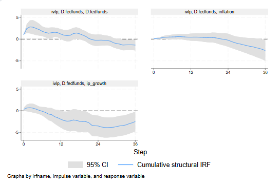
Each panel displays the cumulative response of a variable. The top-left panel shows the response of the interest rate to a shock to interest rate change: the interest rates rises and remains elevated for about one year before returning to its long-run level. The top-right panel shows the cumulative response of inflation, that is, the response of the price level. Prices do not change much for the first two years after the shock, but the response becomes negative by the third year after. The bottom-left panel shows the response of industrial production, which does not change much in the first year after the shock, but becomes negative in the second year, reaching a trough of about −4% after two years.