Bayesian multilevel modeling: Nonlinear, joint, SEM-like

Multilevel models are used by many disciplines to model group-specific effects, which may arise at different levels of hierarchy. Think of regions, states nested within regions, and companies nested within states within regions. Or think hospitals, doctors nested within hospitals, and patients nested within doctors nested within hospitals.

In addition to the standard benefits of Bayesian analysis, Bayesian multilevel modeling offers many advantages for data with a small number of groups or panels. And it provides principled ways to compare effects across different groups by using posterior distributions of the effects. See more discussion here.

bayesmh has a new random-effects syntax that makes it easy to fit Bayesian multilevel models. And it opens the door to fitting new classes of multilevel models. You can fit univariate linear and nonlinear multilevel models more easily. And you can now fit multivariate linear and nonlinear multilevel models!

Think of mixed-effects nonlinear models as fit by menl, or some SEM models as fit by sem and gsem, or multivariate nonlinear models that contain random effects and, as of now, cannot be fit by any existing Stata command. You can now fit Bayesian counterparts of these models and more by using bayesmh.

Let’s see it work

Two-level models

Nonlinear multilevel models

SEM-type models

Joint models of longitudinal and survival data

Multivariate nonlinear growth models

Two-level models

Let’s start simple and fit a few two-level models first.

See Bayesian multilevel models using the bayes prefix. There, we show how to use bayes: mixed and other bayes multilevel commands to fit Bayesian multilevel models. Let’s replicate some of the specifications here using the new random-effects syntax of bayesmh.

We consider the same data on math scores of pupils in the third and fifth years from different schools in Inner London (Mortimore et al. 1988). We want to investigate a school effect on math scores.

Let’s fit a simple two-level random-intercept model to these data using bayesmh. We specify the random intercepts at the school level as U0[school] and include them in the regression specification.

bayesmh requires prior specifications for all parameters except random effects. For random effects, it assumes a normal prior distribution with mean 0 and variance component {var_U0}, where U0 is the name of the random effect. But we must specify the prior for {var_U0}. We specify normal priors with mean 0 and variance 10,000 for the regression coefficients and an inverse-gamma prior with shape and scale of 0.01 for variance components. We specify a seed for reproducibility and use a smaller MCMC size of 1,000.

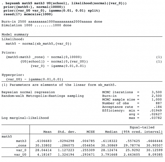
The results are similar to those from bayes: mixed in Random intercepts. We could replicate the same postestimation analysis from that section after bayesmh, including the display and graphs of random effects. In addition to the main model parameters, Bayesian models also estimate all random effects. This is in contrast with the frequentist analysis, where random effects are not estimated jointly with model parameters but are predicted after estimation conditional on model parameters.

Next we include random coefficients for math as c.math3#U1[school]. We additionally need to specify a prior for the variance component {var_U1}. We added to the variance-components list using the inverse-gamma prior.

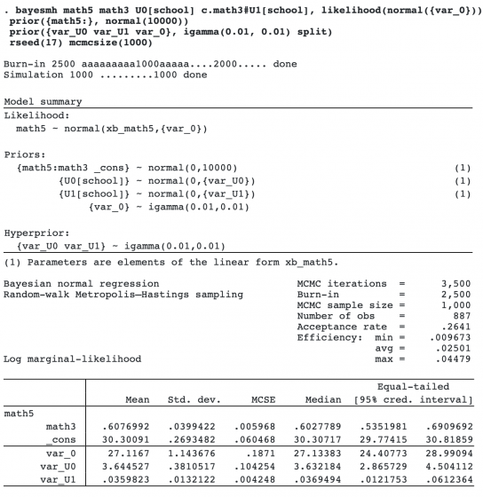
Our results are similar to those from bayes: mixed in Random coefficients.

By default, bayesmh assumes that random effects U0[id] and U1[id] are independent a priori. But we can modify this by specifying a multivariate normal distribution for them with an unstructured covariance matrix {Sigma,m}. We additionally specify an inverse Wishart prior for the covariance {Sigma,m}.

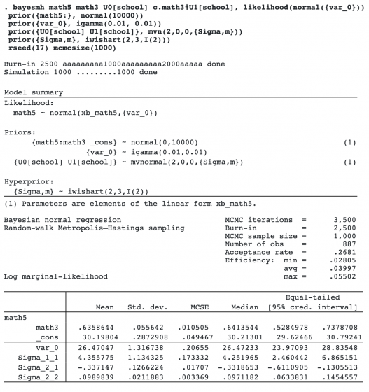
The results are again similar to those from bayes: mixed, covariance(unstructured) in Random coefficients. Just like in that section, we could use bayesstats ic after bayesmh to compare the unstructured and independent models.

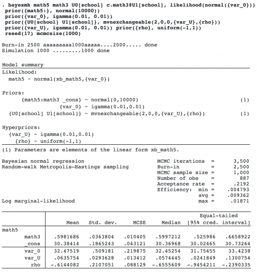
We can also use the new mvnexchangeable() prior option to specify an exchangeable random-effects covariance structure instead of an unstructured. An exchangeable covariance is characterized by two parameters, a common variance and a correlation. We specify additional priors for those parameters.

We could fit other models from Bayesian multilevel models using the bayes prefix by using bayesmh. For instance, we could fit the three-level survival model by using

. bayesmh time education njobs prestige i.female U[birthyear] UU[id<birthyear],
 likelihood(stexponential, failure(failure))
 prior({time:}, normal(0,10000)) prior({var_U var_UU}, igamma(0.01,0.01) split)

and the crossed-effects logistic model by using

. bayesmh attain_gt_6 sex U[sid] V[pid], likelihood(logit)
 prior({attain_gt_6:}, normal(0,10000)) prior({var_U var_V}, igamma(0.01,0.01))

But all these models can be easily fit already by the bayes prefix. In what follows, we demonstrate models that cannot be fit with bayes:.

Nonlinear multilevel models

You can fit Bayesian univariate nonlinear multilevel models using bayesmh. The bayesmh syntax is the same as the menl command that fits classical nonlinear mixed-effects models, except that bayesmh additionally supports crossed effects such as UV[id1#id2] and latent factors such as L[_n].

SEM-type models

You can use bayesmh to fit some structural equation models (SEMs) and models related to them. SEMs analyze multiple variables and use so-called latent variables in their specifications. A latent variable is a pseudo variable that has a different, unobserved, value for each observation. With bayesmh, you specify latent variables as L[_n]. You can use different latent variables in different equations, you can share the same latent variables across equations, you can place constraints on coefficients of latent variables, and more.

Joint models of longitudinal and survival data

You can use bayesmh to model multiple outcomes of different types. Joint models of longitudinal and survival outcomes are one such example. These models are popular in practice because of their three main applications:

1. Account for informative dropout in the analysis of longitudinal data.

2. Study effects of baseline covariates on longitudinal and survival outcomes.

3. Study effects of time-dependent covariates on the survival outcome.

Below, we demonstrate the first application, but the same concept can be applied to the other two.

We will use a version of the Positive and Negative Symptom Scale (PANSS) data from a clinical trial comparing different drug treatmeans for schizophrenia (Diggle 1998). The data contain PANSS scores (panss) from patients who received three treatments (treat): placebo, haloperidol (reference), and risperidone (novel therapy). PANSS scores are measurements for psychiatric disorder. We would like to study the effects of the treatments on PANSS scores over time (week).

A model considered for PANSS scores is a longitudinal linear model with the effects of treatments, time (in weeks), and their interaction and random intercepts U[id].

. bayesmh panss i.treat##i.week U[id], likelihood(normal({var}))

So how does the survival model come into play here?

Many subjects withdrew from this study—only about half completed the full measurement schedule. Many subjects dropped out because of “inadequate for response”, which suggests that the dropout may be informative and cannot be simply ignored in the analysis.

A dropout process can be viewed as a survival process with an informative dropout (infdrop) as an event of interest and with time to dropout as a survival time. Because we have longitudinal data, there are multiple observations per subject. So the dropout time is split into multiple spells according to week and is thus represented by the beginning time (t0) and end time (t1). At the left time point t0, an observation (or a spell) is considered left-truncated. We will assume a Weibull survival model for the dropout process. The dropout is likely to be related to the treatment, so we include it as the predictor in the survival model.

. bayesmh t1 i.treat, likelihood(stweibull({lnp}) failure(infdrop) ltruncated(t0))

One way to account for informative dropout is to include a shared random effect between the longitudinal and survival models that would induce correlation between the longitudinal outcome and the dropout process (Henderson, Diggle, and Dobson 2000).

. bayesmh (panss i.treat##i.week U[id]@1, likelihood(normal({var})))
         (t1 i.treat U[id], likelihood(stweibull({lnp}) failure(infdrop) ltruncated(t0)))

We added random intercepts from the longitudinal model to the survival model. We also constrained the coefficient for U[id] in the first equation to 1. We did this to emphasize that only the coefficient for U[id] in the second equation will be estimated. bayesmh actually makes this assumption automatically by default.

To fit the above model, we need to specify prior distributions for model parameters. We have many parameters, so we may need to specify somewhat informative priors. Recall that Bayesian models, in addition to the main model parameters, also estimate all the random-effects parameters U[id].

If there is an effect of dropout on the PANSS scores, it would be reasonable to assume that it would be positive. So we specify an exponential prior with scale 1 for the coefficient of U[id] in the survival model. We specify normal priors with mean 0 and variance of 1,000 for the constant {panss:_cons} and Weibull parameter {lnp}. We assume normal priors with mean 0 and variance 100 for other regression coefficients. And we use inverse-gamma priors with shape and scale of 0.01 for the variance components.

To improve sampling efficiency, we use Gibbs sampling for variance components and perform blocking of other parameters. We also specify initial values for some parameters by using the initial() option.

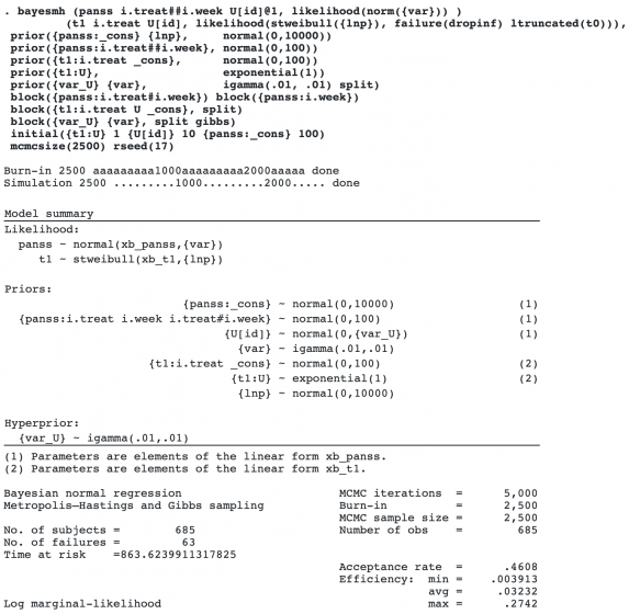
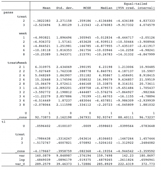
We will not focus on the interpretation of all the results from this model, but we will comment on the coefficient {t1:U} for the shared random intercept. It is estimated to be 0.06, and its 95% credible interval does not contain 0. This means there is a positive association between PANSS scores and dropout times: the higher the PANSS score, the higher the chance of dropout. So, simple longitudinal analysis would not be appropriate for these data.

Multivariate nonlinear growth models

Hierarchical linear and nonlinear growth models are popular in many disciplines, such as health science, education, social sciences, engineering, and biology. Multivariate linear and nonlinear growth models are particularly useful in biological sciences to study the growth of wildlife species, where the growth is described by multiple measurements that are often correlated. Such models often have many parameters and are difficult to fit using classical methods. Bayesian estimation provides a viable alternative.

The above models can be fit by bayesmh using multiple-equation specifications, which now support random effects and latent factors. The equations can be all linear, all nonlinear, or a mixture of the two types. There are various ways to model the dependence between multiple outcomes (equations). For instance, you can include the same random effects but with different coefficients in different equations, or you can include different random effects but correlate them through the prior distribution.

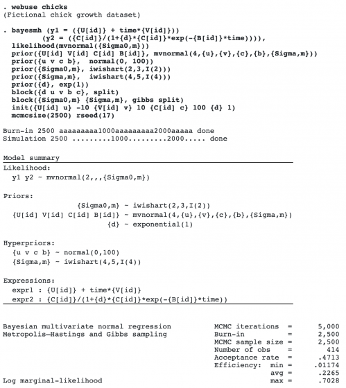
Let’s follow Jones et al. (2005) who applied a Bayesian bivariate growth model to study the growth of black-fronted tern chicks. The growth was measured by wing length y1 and weight y2. A linear growth model is assumed for wing length, and a logistic growth model is assumed for weight.

where d is a fixed parameter, (Ui,Vi,Ci,Bi)∼N(μ,Σ), and (ε1,ε2)∼N(0,Σ0).

There are four random effects at the individual (chick) level: U and V are the intercept and growth rate for the wings. In the equation for y2, we have random effects B and C, which represent the rate and maximum weight. The location parameter is assumed to take the form dC, where d is a constant. (U,V,C,B) follow a multivariate normal distribution with an unstructured covariance. The errors from the two equations follow a bivariate normal distribution.

We use a fictional dataset simulated based on the description in Jones et al. (2005). We fit a bivariate normal model with error covariance {Sigma0,m}. The four random effects are assigned a multivariate normal prior with the corresponding mean parameters and covariance {Sigma,m}. The prior means are assigned normal distributions with mean 0 and variance 100. The covariance matrices are assigned inverse Wishart priors. Parameter d is assigned an exponential prior with scale 1. We use Gibbs sampling for covariance matrices and block parameters to improve efficiency. We also specify initial values, use a smaller MCMC size of 2,500, and specify a random-number seed for reproducibility.

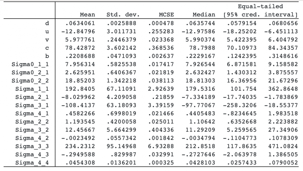
Error covariances and random-effects covariance values are not 0, which suggests that the wing length and weight measurements are related.

We use bayesstats summary to compute correlation estimates.

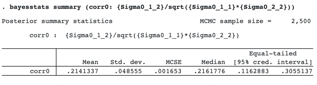
There is a positive correlation, 0.21, between the error terms.

We also compute the correlation between the rate of wing growth and the maximum weight.

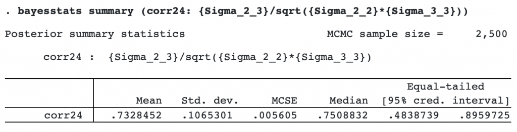
The estimated correlation is 0.73, which is high. The wing length and weight measurements are clearly correlated and should be modeled jointly.