EXAMPLE DATASET: CORRELATION BETWEEN LEGUME CONSUMPTION AND WEIGHT LOSS
The meeting with your future in-laws was a resounding success, thanks in part to your savvy MA of the proportions of vegetarians in the United States. Riding high on this triumph, your future mother-in-law, now brimming with entrepreneurial spirit, is curious about expanding her online restaurant’s menu. This time, she is pondering whether the amount of legume consumption correlates with weight loss. As the resident statistician, you are up to bat again.
You propose conducting an MA of correlations to explore the relationship between legume consumption and weight loss across the United States. With these insights, the online restaurant could spice up its menu to include legume-based recipes to promote a healthier lifestyle, potentially boosting its appeal. Assume you have identified 13 studies.
META-ANALYSIS OF CORRELATION DATA
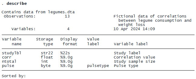
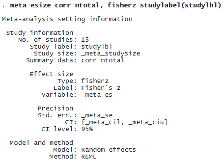
Variables corr and ntotal represent the correlation and the total number of subjects in each study, respectively. We use meta esize to compute the Fisher’s z-transformed correlation for each study. This Fisher’s z–transformation is a variance-stabilizing transformation and is particularly preferable when the correlations are close to −1 or 1.
DECLARE YOUR DATA AS META DATA VIA META ESIZE
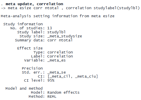
You may instead specify the untransformed (raw) correlation as the effect size using the correlation option. Because the variance of the untransformed correlation depends on the correlation itself, an MA of this effect size tends to assign artificially large weights to studies with correlations close to −1 or 1.
© Copyright 1996–2026 StataCorp LLC. All rights reserved.
FOREST PLOTS AND OTHER META-ANALYSIS TECHNIQUES
Let’s continue with the first specification of meta esize. After computing the effect size of interest and declaring your data as meta data, you may use any MA technique as usual. For example, to construct a forest plot, we type
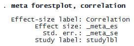
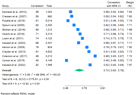
The correlation option specifies that the results be reported as correlations instead of Fisher’s z-values. This is equivalent to applying the hyperbolic tangent transformation using the transform(“Correlation”: tanh) option. The overall (mean) correlation between legume consumption and weight loss is 0.70 with a confidence interval (CI) of [0.63, 0.76].
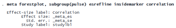
You may conduct a subgroup analysis to investigate whether the correlations differ significantly among the pulse groups:
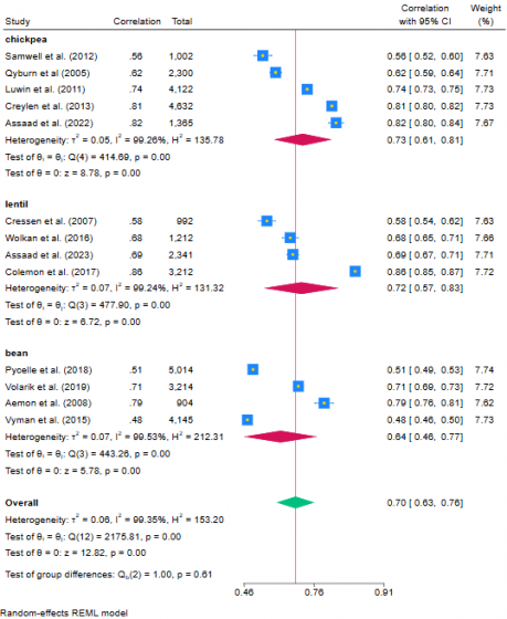
The above forest plots reveal substantive differences within each pulse category. Intriguingly, within each pulse, certain studies show stronger correlations, possibly associated with a supplemental physical activity program alongside the dietary changes. We do not have any evidence that there is a difference between the subgroup correlations (Qb(2)=1.00,p=0.61).
Confident in their potential health benefits, you may advise your mother-in-law to diversify the menu with an array of legume-based dishes without the need to prioritize one pulse type over another in the restaurant recipes.