Below, we use data on the asset prices of 25 fictional companies, along with data on a stock market index sp500. Our data consist of 780 monthly observations containing the end-of-month values for these asset prices.

The first thing we do is to tell Stata we have time-series data using tsset on our date variable, datem:

We have monthly data starting in 1955 with lags defined in one-month increments.

We would like to construct a set of portfolios based on the asset prices in our data and compare them with the market index in our data, the sp500. To create a market return, we type

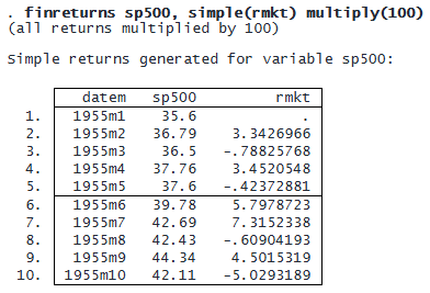
finreturns created a simple return (a percentage change in the asset price). We used the simple() option to give the return the name rmkt rather than the generic default name. Also, we multiplied the return by 100 to obtain percentage changes instead of proportional changes. This simple market return is going to come in handy later on.

We would now like to form a portfolio based on the returns of the other assets in our data. First, we generate simple returns for all of them by typing

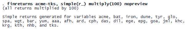
We use the stub r_ to obtain 25 simple returns named r_acme through r_tks corresponding to the price variables acme through tks.

The first portfolio we construct puts equal weight on all the asset returns. We type

The generate() option creates a variable containing the returns of our equally weighted portfolio. Otherwise, we would see only the following output:

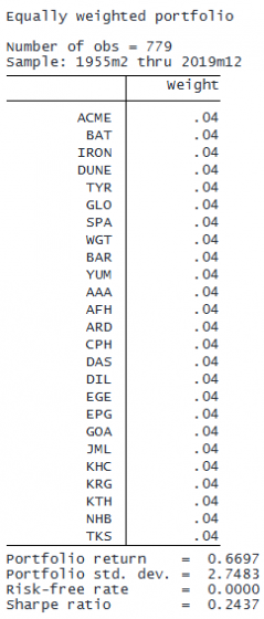
We see that the average portfolio return is 0.67% per month with a standard deviation of 2.75%. Because we did not specify a risk-free rate, these returns are not compared with any benchmark interest rate. Finally, we see the Sharpe ratio. It is a ratio of the mean return to the standard deviation, which gives us a measure of return per unit of risk.

Next, we create two other portfolios, a global minimum-variance portfolio and a portfolio that maximizes the Sharpe ratio.

See Financial portfolio generation to learn more about creating and optimizing portfolios.

We compare the three portfolios we created using finsummarize. We would like to compare their returns, relative to the benchmark market returns we created above.

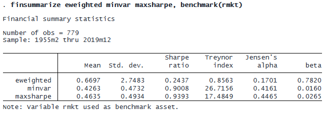
We see that the equally weighted portfolio has the highest average return, but it has more than five times the standard deviation than the other two portfolios.

The Sharpe ratio reflects this by stating that the return per unit of risk is better for our minimum variance and maximum Sharpe ratio portfolios.

The last column is beta, which indicates how much the portfolios vary with the benchmark asset specified in benchmark(). For instance, if beta is negative, it implies that the portfolio does well when the benchmark does poorly (a hedge); if beta is above 1, the portfolio reacts more than proportionally to changes in the benchmark. We see that the equally weighted portfolio moves with the market but not one to one, whereas the other two portfolios with betas around zero seem to be unrelated to the benchmark, meaning that these portfolios are insulated from swings in the benchmark.

The Treynor index is the ratio between mean portfolio return and beta. A higher value implies a high return per unit of risk, where risk is measured in terms of how strongly the portfolio varies with the benchmark.

Jensen’s alpha is the constant in a regression of the asset or portfolio’s returns on the benchmark’s returns. Positive values indicate returns on average that are not captured by beta, that is, returns that can be expected even when the market return is zero. Higher values indicate greater returns.

© Copyright 1996–2026 StataCorp LLC. All rights reserved.

In the table above, underlying Jensen’s alpha and the market beta, there is a CAPM. CAPMs provide an assessment of the performance of an asset with respect to a benchmark market return and a risk-free interest rate (in the example above, it is zero, but often it is the interest rate offered by a central bank, like the federal funds rate in the US). These regressions can be conducted for multiple assets. For our portfolios, we would type

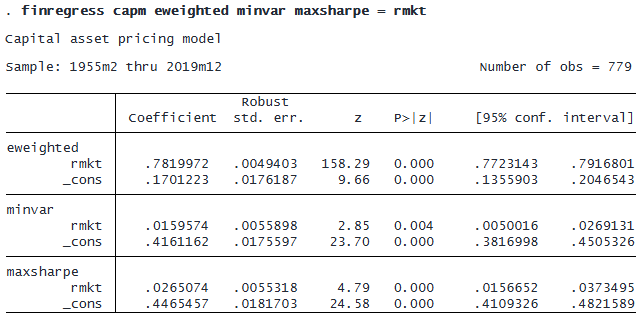
The coefficients on rmkt are the same beta values reported by finsummarize.

CAPM regressions give us information about every asset or portfolio individually. We can also assess the performance of all of them simultaneously. In particular, we can assess how their return is related to risk. To do this, we can use a Fama–MacBeth regression. We would type

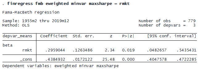
These results indicate that for our three sample portfolios, as beta risk rises by one unit, average return rises by 0.3 percentage points per month. If we wanted to see how average returns are related to beta risk for the whole sample of assets, we would type

See Financial regression to learn more about CAPMs and Fama–MacBeth regression.

We might also be interested in tail behavior. How bad is a bad day with these portfolios? Let’s define a bad day as the negative return (the loss) we would expect to obtain only 5% of the time or less. We can use finvalrisk to assess this threshold using both historical and normal-based methods:

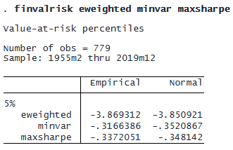
The equally weighted portfolio generates a return of -3.87%, or worse, 5% of the time. Meanwhile, the minimum-variance portfoilo generates a return of -0.32%, or worse, 5% of the time. Thus, the minimum-variance portfolio has much more mild tail behavior than the equally weighted portfolio; that is to say, it is far less risky. Meanwhile, the maximum Sharpe ratio portfolio is comparable with the minimum variance portfolio, albeit slightly riskier, as would be expected.

See Value at risk to learn more about computing VaR.

Of course, there are many other ways to analyze financial data, leveraging tools that are already available in Stata. We could model the variance of our portfolios using autoregressive conditional heteroskedasticity (ARCH) and generalized ARCH (GARCH) models, predict conditional variances, and then visualize them:

We could explore stationarity of the asset returns by using a modified Dickey–Fuller test by typing

Or we can use any other univariate time-series command, such as the arima command to fit an autoregressive integrated moving-average (ARIMA) model.

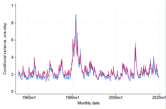
We might also model asset return conditional variance jointly:

Or we can use any multivariate time-series command to study the joint relationship of the asset returns over time.  For instance, we can fit a vector autoregressive model and evaluate the impulse–response functions by typing

We can produce forecasts using the forecast command:

In sum, the arsenal of tools for analyzing financial data at your disposal is large and has expanded.

Read more about financial statistics in the Stata Financial Statistics Reference Manual, and see Financial portfolio generation, Value at risk, and Financial regression.