RANDOM-EFFECTS QUANTILE REGRESSION
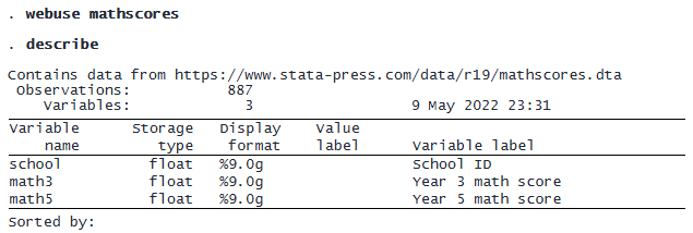
Consider the mathscores dataset, which contains math scores of pupils in the third year (math3) and fifth year (math5) from different schools (school) in Inner London (Mortimore et al. 1988).
We are interested in fitting several Bayesian quantile regressions of math5 on math3 for different quantiles of math5. We also want to include a random intercept at the school level in the model to account for the between-school variability of the math scores.
Let’s first fit a Bayesian random-intercept (panel-data or longitudinal) model for the median. We specify the asymlaplaceq({scale},0.5) likelihood option with a random scale parameter {scale} and a quantile value of 0.5. We use fairly uninformative priors for the coefficients (normal(0,10000)), scale (igamma(0.01,0.01)), and random-intercept variance (igamma(0.01,0.01)). We use blocking to improve the Markov chain Monte Carlo (MCMC) sampling and specify a random seed for reproducibility.
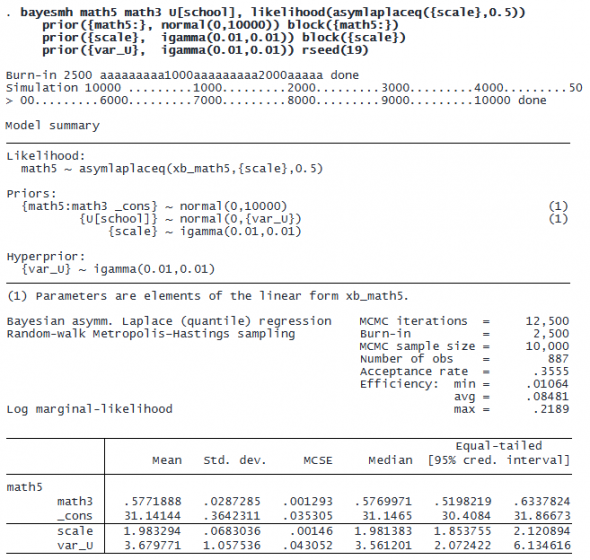
The posterior mean estimate for the math3 coefficient is 0.58, and the variance of the random intercept is 3.68. If we were to fit a Bayesian two-level linear regression that models the conditional mean using the same prior distributions, we would find that its estimates are similar to the estimates obtained from the median regression. A question of interest might be whether the regression coefficients change across quantiles. We can use the estimates from the median regression as a baseline for comparing models for other quantiles.
RANDOM-EFFECTS SIMULTANEOUS QUANTILE REGRESSION
Let’s use bayesmh to fit two Bayesian quantile regressions simultaneously using a two-equation specification. For example, let’s consider the 0.25 and 0.75 quantiles. We label the two regression equations as math5_q25 and math5_q75 to avoid duplication of the outcome variable. Similarly to the previous model, we use uninformative priors for coefficients and variance parameters. We also use a common scale parameter {scale} because the outcome variable is the same in the two equations. The burn-in length is increased to 5,000 to improve sampling adaptation.
© Copyright 1996–2026 StataCorp LLC. All rights reserved.
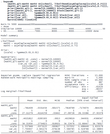
The posterior mean estimates of the math3 coefficient for the 0.25 and 0.75 quantiles are 0.78 and 0.40, respectively, which are above and below the earlier median estimate of 0.58. It appears that the regression slope decreases as the quantile value increases. In particular, we can conclude that math3 is a stronger predictor of the 25th percentile of math5 scores than of the 75th percentile of math5 scores.
MODELING OUTCOMES USING ASYMMETRIC LAPLACE DISTRIBUTION
Finally, we use ALD to examine the skewness (asymmetry) of the math5 variable. For this purpose, we use asymlaplaceq() with a random quantile parameter {tau}. A negative skewness is indicated by {tau} greater than 0.5; positive skewness is indicated by {tau} less than 0.5; and {tau} of 0.5 indicates no skewness, a perfect symmetry. We apply a flat uniform(0, 1) prior for {tau}. We specify a regression model with only a constant term for math5, which corresponds to the location parameter of ALD, and a scale parameter {scale} as in the previous examples.
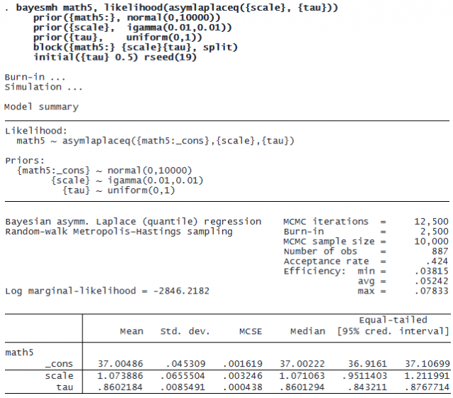
We see that the estimated 95% credible interval of [0.84, 0.88] suggests that {tau} is greater than 0.5, indicating a strong negative skewness. A more formal test for negative skewness can be conducted by using the bayestest interval command.
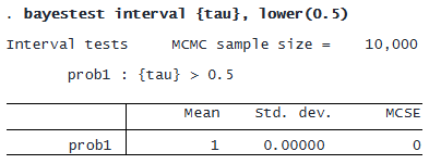
Indeed, the posterior probability of {tau} greater than 0.5 is 1.