Say we are interested in modeling the average rental rate (rent) in each US state as a function of average housing values (hsngval) and the proportion of the population living in urban areas (pcturban). Because average housing values are likely to be endogenous, we include a measure of median family income, faminc, and indicator variables for the region in which each state is located, i.region, as instruments for hsngval. For convenience, we rescale hsngval and faminc to be on a scale similar to rent.
With cfregress, we could reproduce the estimates of a two-stage least-squares (2SLS) IV regression. Whereas 2SLS replaces the endogenous variable in the main regression with fitted values from a first-stage regression, control-function regression keeps the endogenous variable and includes the first-stage residual as a regressor called a control function.
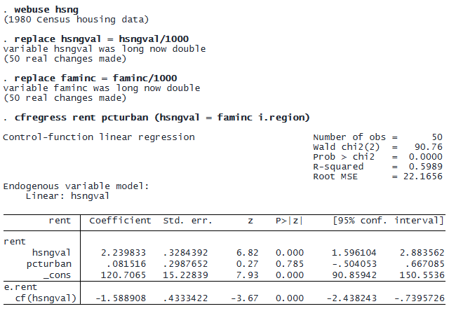
The control function is shown as cf(hsngval) because it is the control function generated from the first-stage model of the endogenous variable hsngval. Control functions enter the main equation, but they are listed under e.rent because we consider them part of the model for the error term.
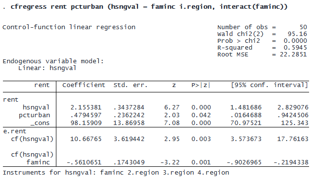
We might suspect that the endogeneity in the model depends not just on the control function but on its interaction with faminc. We include this interaction using the interact() option.
© Copyright 1996–2026 StataCorp LLC. All rights reserved.
The control-function interaction is shown as cf(hsngval)#faminc.
Relative to the first model, there are several changes. We have evidence that the coefficient on pcturban is different from 0, while the coefficient on hsngval is slightly smaller. We also have evidence that the iteraction has a coefficient different from 0, and so should be included in the model.
A joint test of cf(hsngval) and cf(hsngval)#faminc amounts to a test of endogeneity, and we can perform this test by using the postestimation command estat endogenous.
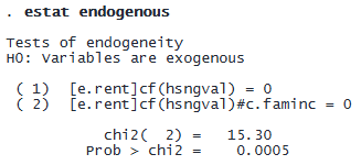
This gives strong evidence for endogeneity. Here we used conventional standard errors, but estat endogenous will conduct an appropriate test after estimation even with robust, cluster–robust, or heteroskedasticity- and autocorrelation-consistent standard errors.
Stata‘s control-function regression commands allow users to specify nonlinear first-stage models for endogenous binary, fractional, or count variables.
For example, we can estimate the effect of having health insurance (ins) on the log of prescription drug expenditure (lndrug) using marital status (married) and employment status (work) as instruments.
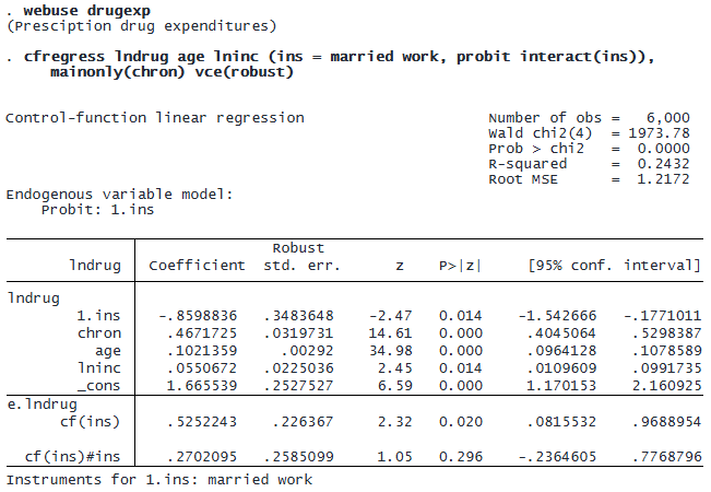
Here we used the probit option within the parentheses to specify a probit model for our first-stage regression. (Note that if we had multiple sets of parentheses, each first-stage regression could have its own model.) We have again included a control-function interaction, and we have also included an indicator for a chronic condition, chron, in the main regression but not the first stage by using the mainonly() option. We requested heteroskedasticity-robust standard errors by specifying the vce(robust) option.
This regression is equivalent to fitting an endogenous treatment-effects model (see Example 2 in [CAUSAL] etregress). What if the outcome is binary? The cfprobit command fits control-function models in the same way except that the model for the main equation is a probit model. Both cfregress and cfprobit allow users the flexibility to specify a large class of models where one or more explanatory variables are endogenous.