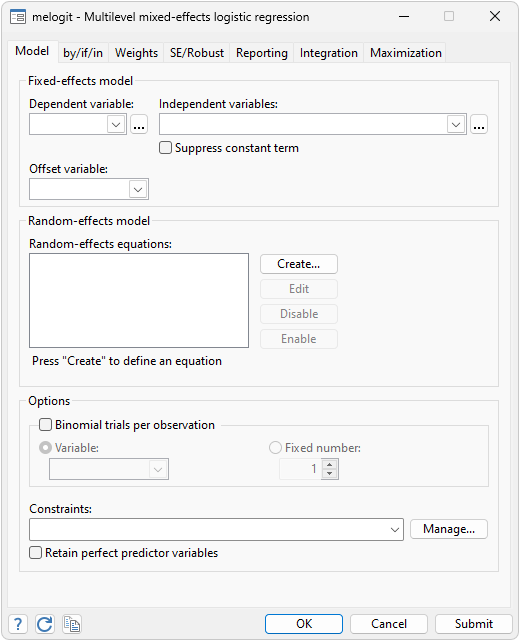
Stata’s meologit allows you to fit multilevel mixed-effects ordered logistic models. A multilevel mixed-effects ordered logistic model is an example of a multilevel mixed-effects generalized linear model (GLM). You can fit the latter in Stata using meglm.
Here we replicate the three-level multilevel model example using the meologit command.
We have student-level data, where students are nested in classes, and classes are nested in schools. Our dependent variable thk is an ordered categorical variable that takes on the values 1, 2, 3, or 4; and we have three explanatory variables: prethk, cc, and tv. We will treat prethk as continuous. cc and tv are binary, and we want to include their interaction in the model. Let’s fit an ordered logistic model:
| Group Variable | No. of Groups | Observations per Group Minimum | Observations per Group Average | Observations per Group Maximum |
| school | 28 | 18 | 57.1 | 137 |
| class | 135 | 1 | 11.9 | 28 |
| thk | Coef. | Std. Err. | z | P>|z| | [95% Conf. Interval] | [95% Conf. Interval] |
| prethk | .4085273 | .039616 | 10.31 | 0.000 | .3308814 | .4861731 |
| 1.cc | .8844369 | .2099124 | 4.21 | 0.000 | .4730161 | 1.295858 |
| 1.tv | .236448 | .2049065 | 1.15 | 0.249 | -.1651614 | .6380575 |
| cc#tv
1 1 |
-.3717699 | .2958887 | -1.26 | 0.209 | -.951701 | .2081612 |
| /cut1 | -.0959459 | .1688988 | -0.57 | 0.570 | -.4269815 | .2350896 |
| /cut2 | 1.177478 | .1704946 | 6.91 | 0.000 | .8433151 | 1.511642 |
| /cut3 | 2.383672 | .1786736 | 13.34 | 0.000 | 2.033478 | 2.733865 |
| school
var (_cons) |
.0448735 | .0425387 | .0069997 | .2876749 | ||
| school>class
var (_cons) |
.1482157 | .0637521 | .063792 | .3443674 |
Our model has two random-effects equations, separated by ||. Our first is a random intercept at the school level, and the second is a random intercept at the class level. The order we listed them matters: class comes after school, meaning that classes are nested within schools. Using the same logic, we could include more levels of nesting.
The output table includes the fixed-effect portion of our model, the estimated cutpoints (because this is an ordered logistic model), and the estimated variance components.


