GOALS

This tutorial explores the estimation of a linear model. After this tutorial you should be able to

• Create linear data using the GAUSS random normal number generator and GAUSS matrix operations.
• Estimate the linear model using matrix operations.
• Estimate the linear model using the ols procedure.

 

INTRODUCTION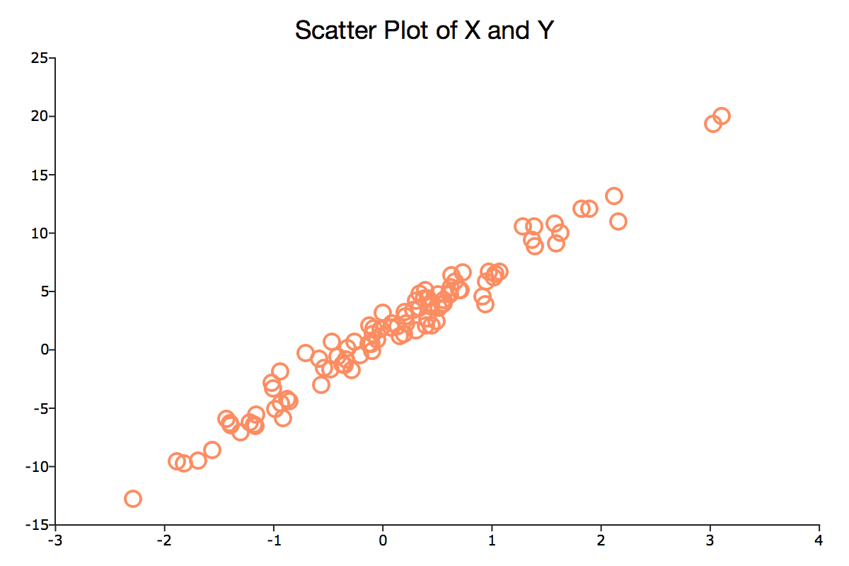 

 

The linear regression model is one of the fundamental workhorses of econometrics and is used to model a wide variety of economic relationships. The general model assumes a linear relationship between a dependent variable, y, and one or more independent variables, x.

 

Y = α + βX

α = intercept

β = slope

 

Note: The graph above was created using the plotScatter procedure. For more information on plotting data see our graph basics tutorial.

 

GENERATE LINEAR DATA

To create our linear data we use a simple univariate linear data generating process

 

 

where ϵi is the random disturbance term. To generate our data we break the process into three simple steps:

 

GENERATE INDEPENDENT DATA

Our first step is to generate a vector with 100 random x values drawn from N(0,1) using the GAUSS command rndn.

 

 // Clear the workspace
 new;

// Set seed to replicate results
 rndseed 23423;

// Number of observations
 num_obs = 100;

// Generate x ~ N(0,1), with
 // 'num_obs' rows and 1 column
 x = rndn(num_obs,1);

 

GENERATE THE ERROR TERM

We will use the same function, rndn, to generate the random disturbances.

 

 // Compute 100 observations of an error term ~ N(0,1)
 error_term = rndn(num_obs,1);

 

GENERATE THE DEPENDENT DATA

Finally, generate y from x and error_term following the data generating process above.

 

 // Simulate our dependent variable
 y = 1.3 + 5.7*x + error_term;

 

Note: The multiplication operator in GAUSS is overloaded to compute matrix multiplication if both inputs are matrices or vectors, and to compute element-by-element (ExE) multiplication if one of the operands is a scalar. Use the dot multiplication operator .*, to compute ExE multiplication of matrices, vectors or multi-dimensional arrays.

ESTIMATE THE MODEL USING MATRIX OPERATIONS 

Using x and y, we can estimate the model parameters and compare our estimates to the true parameters. In order to estimate the constant in our model, we must add a vector of ones to the x matrix. This is easily done using the function ones in GAUSS.

 

Note: The tilde operator, ~, horizontally concatenates two matrices or vectors into one larger matrix.

 

 // Create a new (num_obs x 2) matrix, 'x_mat', where
 // the first column is all ones
 x_mat = ones(num_obs, 1) ~ x;

 

We can now estimate the two parameters of the model, the constant and slope coefficient, using our x matrix and y vector :

 

© 2025 Aptech Systems, Inc. All rights reserved.

 

 //Compute OLS estimates, using matrix operations
 beta_hat = inv(x_mat'x_mat)*(x_mat'y);

print beta_hat;

 

The above print statement should return the following output:

 

1.2795490
5.7218389

 

ESTIMATE THE MODEL USING  ols FUNCTION 

Above we used matrix operations to calculate the parameters of the model. However, GAUSS includes a built-in function ols which will perform the same estimation for us. The function will find the parameter models and provide several model diagnostics. ols takes the following three inputs:

 

• dataset
  • String, name dataset to use for regression. Use an empty string, "", if x and y are matrices
• x
  • Matrix of independent variable for regression, or string with variable names
• y
  • Vector of dependent variables, or string with name of independent variable

 

In our case, we will use the x and y data which we created. As these are not related to any dataset, we can enter a blank string, "" for the dataset input. Furthermore, rather than sending the output to any variables, we will simply print the output to screen using the command call.

 

call ols("", y, x);

 

Which should print a report similar to the following:

 

Valid cases:                100      Dependent variable:                   Y
Missing cases:                0      Deletion method:                   None
Total SS:              3481.056      Degrees of freedom:                  98
R-squared:                0.969      Rbar-squared:                     0.969
Residual SS:            107.205      Std error of est:                 1.046
F(1,98):               3084.149      Probability of F:                 0.000

                        Standard               Prob   Standardized  Cor with
Variable    Estimate     Error     t-value     >|t|     Estimate    Dep Var
-----------------------------------------------------------------------------
CONSTANT    1.27955    0.105343   12.14651     0.000       ---         ---
X1          5.72184    0.103031   55.53512     0.000    0.984481    0.984481

CONCLUSION

Congratulations! You have:

• Used matrix operations to generate linear data.
• Estimated an OLS model using matrix operations.
• Estimates an OLS model using ols.

 

For convenience, the full program text is reproduced below.

 

The next tutorial describes using the estimated parameters to predict outcomes and compute residuals.

 

// Clear the workspace
 new;

// Set seed to replicate results
 rndseed 23423;

// Number of observations
 num_obs = 100;

// Generate x ~ N(0,1), with
 // 'num_obs' rows and 1 column
 x = rndn(num_obs,1);

// Compute 100 observations of an error term ~ N(0,1)
 error_term = rndn(num_obs,1);

// Simulate our dependent variable
 y = 1.3 + 5.7*x + error_term;

// Create a new (num_obs x 2) matrix, 'x_mat', where
 // the first column is all ones
 x_mat = ones(num_obs, 1) ~ x;

// Compute OLS estimates, using matrix operations
 beta_hat = inv(x_mat'x_mat)*(x_mat'y);

print beta_hat;

call ols("", y, x);