INTRODUCTION
Traditionally, one selects a model and perform inference and prediction conditional on this model. The results obtained typically do not account for the uncertainty in selecting a model and thus may be overly optimistic. They may even be incorrect if the selected model is substantially different from the true data-generating model (DGM). In some applications, researchers may have strong theoretical or empirical evidence about the DGM. In other applications, usually of complex and unstable natures, such as those in economics, psychology, and epidemiology, choosing one reliable model can be difficult.
Instead of relying on just one model, model averaging averages results over multiple plausible models based on the observed data. In BMA, the “plausibility” of the model is described by the posterior model probability (PMP), which is determined using the fundamental Bayesian principles—the Bayes theorem—and applied universally to all data analyses.
BMA can be used to account for model uncertainty when estimating model parameters and predicting new observations to avoid overly optimistic conclusions. It is particularly useful in applications with several plausible models, where there is no one definitive reason to choose a particular model over the others. But even if choosing a single model is the end goal, users can find BMA beneficial. It provides a principled way to identify important models and predictors within the considered classes of models. Its framework allows one to learn about interrelations between different predictors in terms of their tendency to appear in a model together, separately, or independently. It can be used to evaluate the sensitivity of the final results to various assumptions about the importance of different models and predictors. And it provides optimal predictions in the log-score sense.
THE BMA SUITE
In a regression setting, model uncertainty amounts to the uncertainty of which predictors should be included in a model. One can use bmaregress to account for selection of predictors in a linear regression. It explores the model space either exhaustively with the enumeration option, whenever feasible, or by using the Markov chain Monte Carlo (MCMC) model composition (MC3) algorithm with the sampling option. It reports various summaries of the visited models and included predictors and of posterior distributions of model parameters. It allows researcher to specify groups of predictors to be included or excluded together from a model and those that are included in all models. It provides various prior distributions for models in the mprior() option and for the g parameter, which controls shrinkage of regression coefficients toward zero, in the gprior() option. It also supports factor variables and time-series operators and provides several ways for handling interactions during estimation by using the heredity() option.
| Command | Description |
|---|---|
|
bmacoefsample |
Posterior samples of regression coefficients |
|
bmagraph pmp |
model-probability plots |
|
bmagraph msize |
model-size distribution plots |
|
bmagraph varmap |
variable-inclusion maps |
|
bmagraph coefdensity |
coefficient posterior density plots |
|
bmastats models |
posterior model and variable-inclusion summaries |
|
bmastats msize |
model-size summary |
|
bmastats pip |
posterior inclusion probabilities (PIPs) for predictors |
|
bmastats jointness |
jointness measures for predictors |
|
bmastats lps |
log predictive-score (LPS) |
|
bmapredict |
BMA predictions |
|
bayesgraph |
Bayesian graphical summaries and convergence diagnostics |
|
bayesstats summary |
Bayesian summary statistics for model parameters and their functions |
|
bayesstats ess |
Bayesian effective sample sizes and related statistics |
|
bayesstats ppvalues |
Bayesian predictive p-values |
|
bayespredict |
Bayesian predictions |
There are many supported postestimation features, which also include some of the standard Bayesian postestimation features.
BMA IN ACTION!
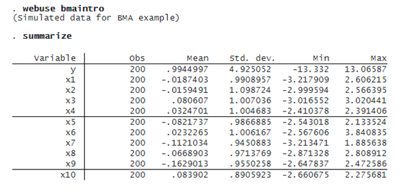
Below, we provide a tour of some bma features using a toy dataset. This dataset contains n=200 observations, p=10 orthogonal predictors, and outcome y generated as
y=0.5+1.2×x2+5×x10+ϵ
where ϵ∼N(0,1) is a standard normal error term.
MODEL ENUMERATION
We use bmaregress to fit a BMA linear regression of y on x1 through x10.
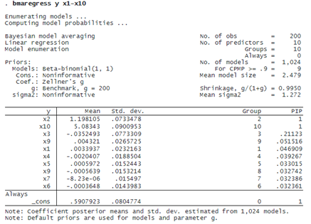
With 10 predictors and the default fixed (benchmark) g-prior, bmaregress uses model enumeration and explores all 2^10=1,024 possible models. The default model prior is beta-binomial with shape parameters of 1, which is uniform over the model size. A priori, our BMA model assumed little shrinkage of regression coefficients toward zero because g/(1+g)=0.9950 is close to 1.
bmaregress identified x2 and x10 as highly important predictors—their posterior inclusion probabilities (PIPs) are essentially 1. The posterior mean estimates of their regression coefficients are, respectively, 1.2 (rounded) and 5.1 and are very close to the true values of 1.2 and 5. All other predictors have much lower PIPs and coefficient estimates close to zero. Our BMA findings are consistent with the true DGM.
Let’s store our current estimation results for later use. As with other Bayesian commands, we must save the simulation results first before we can use estimates store to store the estimation results.
. bmaregress, saving(bmareg)
note: file bmareg.dta saved.

. estimates store bmareg
CREDIBLE INTERVALS
bmaregress does not report credible intervals (CrIs) by default, because it requires a potentially time-consuming simulation of the posterior sample of model parameters. But we can compute them after estimation.
We first use bmacoefsample to generate an MCMC sample from the posterior distribution of model parameters, which include regression coefficients. We then use the existing bayesstats summary command to compute posterior summaries of the generated MCMC sample.
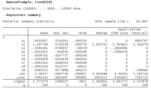
The 95% CrI for the coefficient of x2 is [1.05, 1.34], and the one for x10 is [4.9, 5.26], which is consistent with our DGM.
INFLUENTIAL MODELS
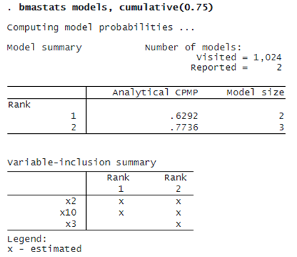
The BMA coefficient estimates are averaged over 1,024 models. It is important to investigate which models are influential. We can use bmastats models to explore the PMPs.
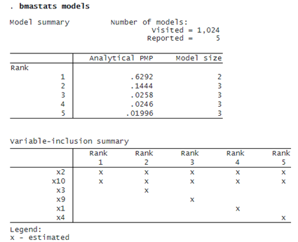
Not surprisingly, the model that contains both x2 and x10 has the highest PMP of about 63%. In fact, the top two models correspond to a cumulative PMP of about 77%:
We can use bmagraph pmp to plot the cumulative PMP.
. bmagraph pmp, cumulative

© Copyright 1996–2024 StataCorp LLC. All rights reserved.
The command plots the first 100 models by default, but you can specify the top() option if you would like to see more models.
IMPORTANT PREDICTORS
We can explore the importance of predictors visually by using bmagraph varmap to produce a variable-inclusion map.
. bmagraph varmap

Computing model probabilities ...

x2 and x10 are included in all top 100 models, ranked by PMP. Their coefficients are positive in all models.
MODEL-SIZE DISTRIBUTION
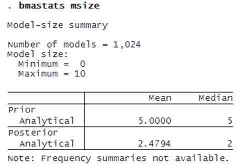
We can explore the complexity of our BMA model by using bmastats msize and bmagraph msize to explore the prior and posterior model-size distributions.
. bmagraph msize

The prior model-size distribution is uniform over the model size. The posterior model-size distribution is skewed to the left with the mode of about 2. The prior mean model size is 5 and the posterior one is 2.48. So, based on the observed data, BMA tends to favor smaller models with roughly two predictors, on average, compared with our a priori assumption.
POSTERIOR DISTRIBUTIONS OF COEFFICIENTS
We can use bmagraph coefdensity to plot posterior distributions of regression coefficients.
. bmagraph coefdensity {x2} {x3}, combine

These distributions are mixtures of a point mass at zero corresponding to the predictor’s probability of noninclusion and a continuous density conditional on the inclusion. For the coefficient of x2, the probability of noninclusion is negligible, so its posterior distribution is essentially a continuous, fairly symmetric density centered at 1.2. For the coefficient of x3, in addition to the conditional continuous density, there is a red vertical line at zero corresponding to the posterior noninclusion probability of roughly 1-.2 = 0.8.
BMA PREDICTION
bmapredict produces various BMA predictions. For instance, let’s compute the posterior predictive means.
. bmapredict pmean, mean
note: computing analytical posterior predictive means.
We can also compute predictive CrIs to estimate uncertainty about our predictions. (This is not available with many traditional model-selection methods.) Note that these predictive CrIs also incorporate model uncertainty. To compute predictive CrIs, we must save the posterior MCMC model-parameter sample first.
. bmacoefsample, saving(bmacoef)
note: saving existing MCMC simulation results without resampling; specify
      option simulate to force resampling in this case.
note: file bmacoef.dta saved.

. bmapredict cri_l cri_u, cri rseed(18)
note: computing credible intervals using simulation.

Computing predictions ...
We summarize the predicted results:
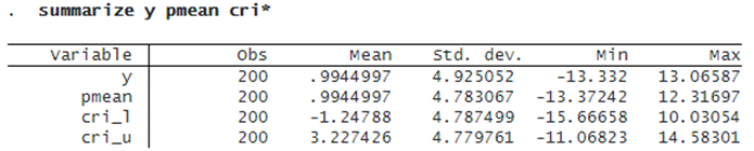
The reported averages over observations for predictive means and lower and upper 95% predictive CrI bounds look reasonable relative to the observed outcome y.
INFORMATIVE MODEL PRIORS
One of the strengths of BMA is the ability to incorporate prior information about models and predictors. This allows us to investigate the sensitivity of the results to various assumptions about the importance of models and predictors. Suppose that we have reliable information that all predictors except x2 and x10 are less likely to be related to the outcome. We can specify, for example, a binomial model prior with low prior inclusion probabilities for these predictors.
To compare the out-of-sample performance of the BMA models later, we randomly split our sample into two parts and fit the BMA model using the first subsample. We also save the results from this more informative BMA model.
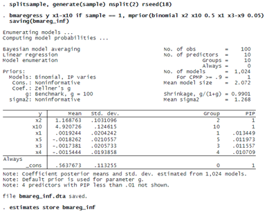
The effect of this model prior is that the PIP of all unimportant predictors is now less than 2%.
Note that when we select one model, we are essentially fitting a BMA model with a very strong prior that all selected predictors must be included with a probability of 1. For instance, we can force bmaregress to include all variables in the model:
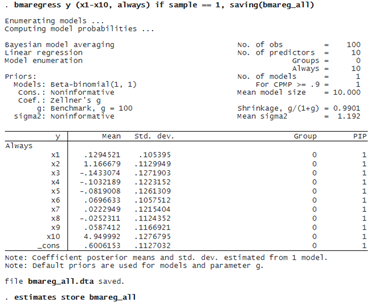
PREDICTIVE PERFORMANCE USING LPS
For comparison of the considered BMA models, we refit our default BMA model using the first subsample and store the estimation results.
. qui bmaregress y x1-x10 if sample == 1, saving(bmareg, replace)
. estimates store bmareg
We can compare the out-of-sample predictive performance of our BMA models by using bmastats lps to compute the log predictive-score (LPS) for out-of-sample observations.
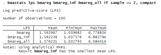
The more informative bmareg_inf model has a slightly smaller mean LPS, but the LPS summaries for all models are very similar. See [BMA] bmastats lps for how to compare the BMA model performance by using cross-validation.
CLEANUP
We generated several datasets during our analysis. We no longer need them, so we erase them at the end. But you may decide to keep them, especially if they correspond to a potentially time-consuming final analysis.
. erase bmareg.dta
. erase bmacoef.dta
. erase bmareg_inf.dta
. erase bmareg_all.dta