HETEROGENEOUS DIFFERENCE IN DIFFERENCES (DID) IN ACTION!
We would like to know if a school-district-level program, Healthy Habits, reduces students’ body mass index (BMI) in the school district. We have fictional data on the Healthy Habits program. This program incorporates more exercise time and augments the intake of fruits and vegetables. Our data are at the school district level and include information on whether a school participates in the program, hhabit, and the BMI of students in the district, bmi. We have repeated samples of students ages 11 to 14 from 40 school districts from 2013 to 2021.
For the outcome model, we believe that the mother’s education, medu, is a good predictor of the health habits of children. We also believe that participation in sports, sports, affects bmi. Finally, we control for whether the student is a girl to account for behavioral differences and differences in body types of boys and girls at this age.
For the treatment model, we use the number of parks in the district (parksd) to model hhabit. We conjecture that school districts with more parks consider exercise spaces more important in their urban planning than those with fewer parks. These districts are therefore more amenable to the Healthy Habits program.
We use the aipw estimator to model both the outcome and the treatment. The aipw estimator has a double-robustness property, implying that only one of the outcome model or the treatment model needs to be correctly specified to obtain consistent estimates.
We fit the following model:
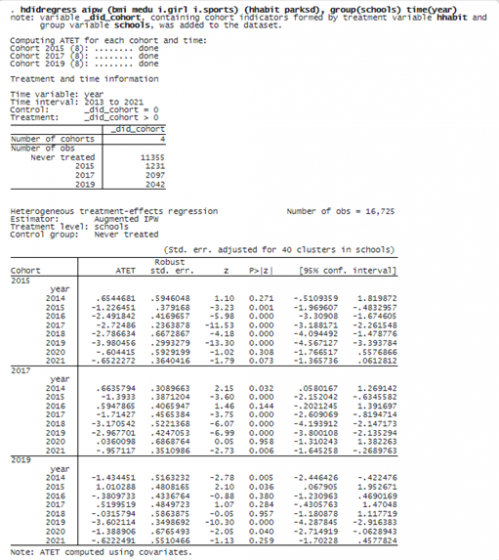
We specified the outcome model in the first set of parentheses and the treatment model in the second set of parentheses. We also specified option group(schools) to define that treatment occurs at the school level and to identify schools as the clustering variable. Finally, we specified a time variable year in option time().
The note below the command indicates that the categorical variable _did_cohort is generated with cohort information. Units in the same cohort start the treatment at the same time. We see that there are three cohorts in our data: 2015, 2017, and 2019. In addition, we see that 11,355 observations are never treated. The time variable year ranges from 2013 to 2021.
The estimation table reports the ATET for each cohort in each year. For example, for the cohort 2015 in the year 2016, the ATET estimate is –2.5, which implies the Healthy Habits program, on average, reduces BMI by 2.5 for students in a district of the 2015 cohort in 2016 relative to the scenario where the district does not participate. The other estimates can be interpreted similarly.
It is difficult to see the trends in ATETs just by looking at all the ATETs estimates. We can use estat atetplot to visualize the time profile of ATETs for each cohort. We specify option sci to show the simultaneous confidence bands guaranteed to cover the true values of ATETs across all the cohorts and time with a predefined probability level.
. estat atetplot, sci
© Copyright 1996–2025 StataCorp LLC. All rights reserved.

After fitting the model, we can use estat aggregation to aggregate the ATETs within cohort, time, and exposure to treatment. It provides a summary of different aspects of ATETs. For example, we use estat aggregation, cohort to summarize the ATETs of each cohort within time. We also specify option graph to obtain a graph of aggregations in addition to the tabular output.
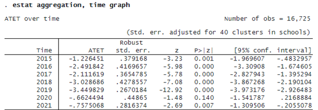

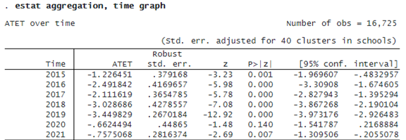
If we want to summarize ATETs within time, we specify option time with estat aggregation.

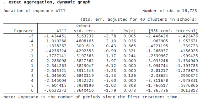
Finally, if we want to summarize ATETs over different lengths of exposure to treatment, we specify option dynamic.