Lasso with clustered data

You can now account for clustered data in your lasso analysis. Ignoring clustering may lead to incorrect results in the presence of correlation between observations within the same cluster. But with Stata’s lasso commands—both those for prediction and those for inference—you can now obtain results that account for clustering.

With lasso commands for prediction, you simply add the cluster() option. For instance, type

. lasso linear y x1-x5000, cluster(idcode)

to account for possible correlation between observations with the same idcode during model selection. You can do this with lasso models other than linear, such as logit or Poisson, and with variable-selection methods other than lasso, such as elastic net and square-root lasso.

With lasso commands for inference, you add the vce(cluster) option. For instance, type

. poregress y x1, controls(x2-x5000) vce(cluster idcode)

to produce cluster–robust standard errors that account for clustering in idcode using partialing-out lasso for linear outcomes. The vce(cluster) option is supported with all inferential lasso commands, including the new command for treatment-effects estimation with lasso.

Let’s see it work

We want to fit a linear-lasso model for the log of wages (ln_wage) using a set of variables and their second-order interactions. We have data on the individual’s age, age; work experience, experience; job tenure, tenure; whether the individual lives in a rural area, rural; if they live in the South, south; and if they have no college education, nocollege. We want a good prediction of the log of wages given these controls.

We have repeated observations of individuals over time; we have clustered data. Each individual is identified by idcode.

We define the global macro $vars as variables and $controls as the full list of control variables.

. global vars c.(age tenure experience) i.(rural south nocollege)

. global controls ($vars)##($vars)

We fit the lasso model and specify option cluster(idcode) to account for clustering, and we specify option rseed(1234) to make the results reproducible.

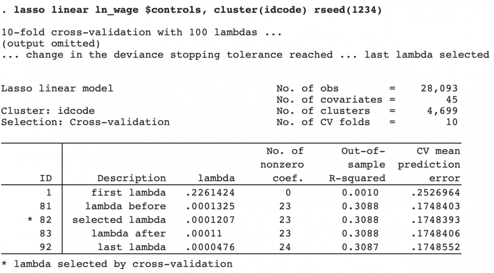
There are 4,699 clusters. Behind the scenes, the cross-validation procedure draws random samples by idcode to arrive at the optimal lambda.

We could now use the predict command to get predictions of ln_wage.

Suppose we are not interested solely in prediction. Say we want to know the effect of job tenure (tenure) on log wages (ln_wage). All the other variables are treated as potential controls, which lasso may include or exclude from the model. Lasso for inference allows us to obtain the estimate of the effect of tenure and its standard error. Because individuals are correlated over time, we would like to use cluster–robust standard errors at the idcode level. We fit a linear model with double-selection lasso methods by using the dsregress command.

First, we define the global macro $vars2 as the uninteracted control variables, and we interact them to form the complete set of controls in $controls2.

. global vars2 c.(age experience) i.(rural south nocollege)

. global controls2 ($vars2)##($vars2)

To fit the model and estimate cluster–robust standard errors, we use dsregress and specify the option vce(cluster idcode).

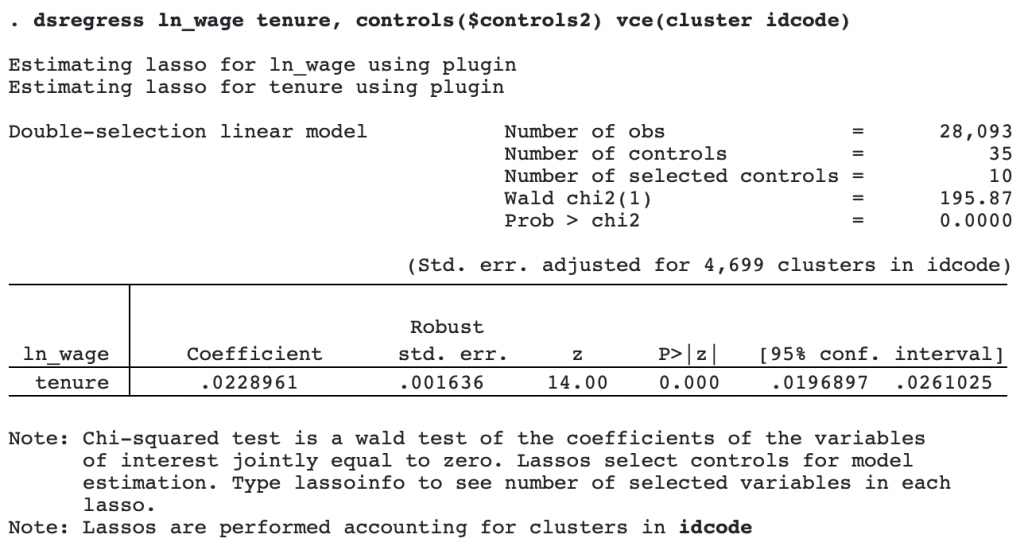
The .02 point estimate means that an increase of one year in job tenure would increase the log of wage by .02. The standard-error estimate is robust to the correlated observations within the cluster.