LOCAL PROJECTIONS FOR IMPULSE–RESPONSE FUNCTIONS IN ACTION
We have quarterly data on inflation, the output gap, and the Federal funds rate.

We start by estimating the impulse–response function of a univariate model of the output gap.
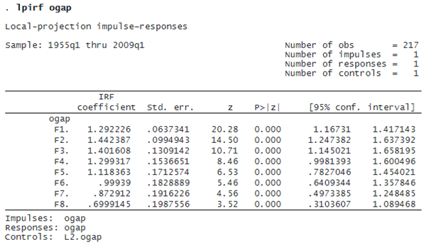
Each coefficient is the response to an impulse (shock) to the output gap at the specified number of periods ahead. On impact, the effect of the shock is one unit. After one period (F1.ogap), the output gap rises further to 1.29. Then peaks in the second period at 1.44. The response falls to 0.70 eight periods after a shock.
More interesting models arise when there are multiple variables, in which case we can assess the effect of a shock to one variable on another. We combine the lpirf command with the irf suite of commands to estimate, then graph, orthogonalized impulse–response functions.
. quietly lpirf inflation ogap fedfunds, lags(1/12) step(24)
. irf set myirfs.irf, replace
. irf create model1
. irf graph oirf, yline(0)

The first row plots the response to a federal funds rate shock; the second row plots the response to an inflation shock; and the final row plots the response to an output gap shock. An unexpected rise in interest rates leads inflation and output to both fall over the subsequent quarters, with inflation’s response reaching a trough around 12 steps (3 years) after the impulse and with output’s response reaching a trough around 8 steps (2 years) after the impulse. The inflation shock pushes inflation and output in opposite directions, and the interest rate rises mildly in response. The output shock leads inflation and the interest rate to both rise.
In this example, we have a monthly dataset on the logarithm of the industrial production index, the logarithm of the consumer price index, and a measure of exogenous monetary shocks from Romer and Romer (2004) and updated in Wieland and Yang (2020).
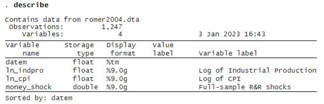
We are interested in the responses of industrial production and inflation to a monetary shock. We treat industrial production and inflation as endogenous and treat the monetary shock as exogenous. We fit two models: a local‐projection model and a vector autoregression (VAR) model.
. irf set comparemodels.irf, replace
. quietly lpirf indpro inflation, lags(1/12) exog(L(0/12).money_shock)
. irf create lpmodel
. quietly var indpro inflation, lags(1/12) exog(L(0/12).money_shock)
. irf create varmodel
. irf graph dm, impulse(money_shock) irf(lpmodel varmodel)
The dynamic multipliers from the local‐projection and VAR models are

The top row shows the results of the local‐projection model. The bottom row shows the results of the VAR model, treating the money shock as exogenous.
Both the local‐projection and the VAR model show a slight increase in the price level after a monetary shock, peaking around 24 months after the shock and declining thereafter. Both models indicate that industrial production falls after a monetary shock, with a trough occurring around 24 months after the shock. The local-projection IRFs and VAR model IRFs provide similar results over short horizons, but begin to diverge at longer horizons. Local projections provide more flexibility in long-run responses by estimating them directly. And local projections are much faster to compute.