EXTENDED REGRESSION MODELS FOT PAMEL FOT PANEL-DATA/MULTILEVEL MODELS
Stata’s Extended Regression Models (ERMs) now support panel data.
ERMs were added last release to Stata. They fit models with problems.
By models, we mean linear regression and interval regression for continuous outcomes, probit for binary outcomes, and ordered probit for ordered outcomes.
By problems, we mean any combination of endogenous and exogenous sample selection, endogenous covariates (unobserved confounders), and nonrandom treatment assignment.
New this release is that ERMs handle yet another problem—panel data (also known as longitudinal data or two-level multilevel data).
Random effects are included in each equation by default. Random effects are correlated; you can omit specific random effects, and you can test the correlations.
Other commands in Stata can fit models with any of the problems listed. ERMs can handle any combination of the above problems and can fit models with continuous, interval, binary, and multiple outcomes.
Discipline disambiguation
The problems that ERMs handle go by different names in different disciplines. Here is a list of the synonyms.
Endogenous and exogenous sample selection
Trials with informative dropout
Outcomes missing not at random (MNAR)
Nonignorable nonresponse
Selection on unobservables
Heckman selection
Endogenous covariates (unobserved confounders)
Bias due to unmeasured confounding
Simultaneous causality in linear models
Measurement error
Causal inference
Nonrandom treatment assignment
Causal inference
Average causal effects (ACEs)
Average treatment effects (ATEs)
Panel data
Longitudinal data
Two-level multilevel data
ERM syntax and workflow
You should be interested in ERMs’ new features if you fit cross-sectional time-series models, two-level multilevel models, or panel-data models.
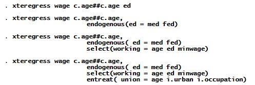
Say you are interested in modeling wages and have repeated observations on individuals over the years 2011–2018. You might model their wages as a linear function of age, age squared, and education. There are two traditional ways you could fit this model in Stata:
. xtreg  wage  c.age##c.age ed

. meglm  wage  c.age##c.age ed || :id
xtreg is Stata’s command for handling panel data.
meglm is Stata’s command for handling multilevel and hierarchical data.
Both work because panel data are a special case of multilevel data. Panel data are multilevel data with two levels.
Or you could fit the model with Stata’s new ERMs xteregress command:
. xteregress wage c.age##c.age ed
All will produce equivalent results, and all will incorporate individual heterogeneity, a.k.a. random effects. It does not matter which command you use if your data are as we have described them.
If, however, your data suffer from any of the problems we listed above, you need to use xteregress. We say problems with your data, but whether the problems are specific to your data or a feature of reality makes no difference when it comes to fitting the model. The sources of the problems — they can vary problem by problem — matter for how you interpret and test the results. Another feature of ERMs is that they provide the tools you need for interpretation.
Consider panel data and the model
. xteregress wage c.age##c.age ed
To show you how easy ERMs are to use, we are going to sequentially introduce problems and solve them. By solve, we mean that we will obtain estimates that any of the above commands would have produced if only the data did not have the problems we are about to add.
We are about to play fast and loose with problems and their solutions. Forgive us. We write software. We want to show you how easy ERMs make it to implement solutions. For the problems that you find, you will certainly be more thoughtful about the solutions that you implement than we are about to be.
First problem: Endogeneity
It would certainly be reasonable to suspect that educational attainment is correlated with unobservable components not included in the data and perhaps not even conceptually observable in reality. And it would be reasonable to assume that those same unobservables might positively affect wages. For instance, having a good home background might prepare one better for the world, leading to higher educational attainment and higher wages. Anyway, whatever the cause of the problem, you decide to model each person’s educational attainment as a function of their mother’s and father’s educational attainment, med and fed. Here is how you would do that:
. xteregress wage c.age##c.age,
                     endogenous(ed = med fed)
What we did was move ed from the list of exogenous variables before the comma and into the endogenous() option. ed will still be included in the model for wage but as an endogenous variable. Its reported coefficient will be adjusted for the confounding or endogeneity, just as if the data did not have the problem.
First problem solved.
Second problem: Endogenous sample selection.
You observe wages in your data only for those who work. What if those who do not work would have a wage that was systematically higher or lower? It could go either way. People with higher wages would find working more enticing. On the other hand, people with lower wages will have a greater need to work. You decide to model whether a person works as a function of age, education, and minimum wage so that the bias, whichever way it goes, can be washed away.
. xteregress wage c.age##c.age,
                      endogenous( ed = med fed)
                      select(working = age ed minwage)
Second problem solved.
And this second problem was solved even though education affects the choice to work and is itself endogenous!
Third problem: Endogenous treatment assignment
Some people in the data belong to unions. Union effects on wages and membership might not be random. If it is not, we have endogenous treatment assignment. Assume that. The solution would be to model union membership.
. xteregress wage c.age##c.age,
                      endogenous( ed = med fed)
                      select(working = age ed minwage)
                      entreat( union = age i.urban i.occupation)
Third problem solved.
We will stop now. We have only scratched the surface of what ERMs can do.
Let’s see it work
We discussed four models:
Here is the second one:
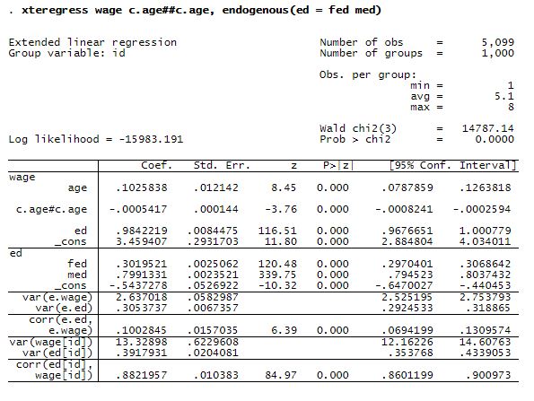
here are six sections in the above output.
wage. This section shows the wage equation. Here, ed is washed of its endogeneity.
ed. This section shows the ed equation used to wash ed of its endogeneity.
The remaining sections present information about the residuals and random effects. So let’s tell you how to read the encoded names.
| var(…) | means variance of … |
| corr(…, …) | means correlation of … and … |
| e.wage | is the residual on the wage equation |
| e.ed | is the residual on the ed equation |
| wage[id] | is the random effect in the wage equation |
| ed[id] | is the random effect in the ed equation |
e.wage and e.ed are the overall residuals. They vary over time and by person.
The random effects wage[id] and ed[id] are residuals too, but they are a different kind of residual. They vary across persons, but are constant within persons. That is why they include the subscript [id]. id is the person identification number.
We wondered whether education was endogenous. Were we right to worry? corr(e.ed,e.wage) and corr(ed[id],wage[id]) can answer that question. Correlation in either is endogeneity but of different kinds.
The striking correlation is 0.88 for the random effects. It is huge. It is whoppingly significant at 85 standard deviations away from what might be observed randomly. And it means that unobservables that increase wages increase educational attainment.