NLME models - TStat

NLME MODELS WITH LAGS, LEADS, AND DIFFERENCES: GROWTH MODELS, MULTIPLE-DOSE PK MODELS, AND MORE

Existing command menl has new features for fitting nonlinear mixed-effects models (NLMEMs) that may include lag, lead (forward), and difference operators. One important class of such models is the class of pharmacokinetic (PK) models and, specifically, multiple-dose PK models. menl‘s new features can also be used to fit other models, such as certain growth models and time-series nonlinear multilevel models.

Let’s see it work

Growth models

Multiple-dose PK models

Other features

Growth models

Growth models based on difference equations are often used to model animal growth. For instance, Andrews (1982) used the so-called logistic-by-weight model to model the growth of small lizards. Wright et al. (2013) applied this model to study the length of brown anole lizards. The authors also extended the model to account for the between-lizard variation by including random effects.

Inspired by the above studies, we created our own fictional data on lengths of small lizards. In what follows, we will use menl to fit a random-effects logistic-by-weight model to these data.

First, let’s take a quick look at the data. We list the observations for the first two lizards.

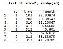
Lizards were captured and their length measured. Then, they were marked and released. After that, the lizards were recaptured at different times, and their length was recorded again. Variable time contains the number of days since the beginning of the study, and length records the length (in mm) of lizards.

The interval version of the random-effects logistic-by-weight model can be defined as

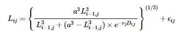
where $L_{i j}$ is the length of lizard $j$ at time $i$ and $D_{i j}$ is the difference in days between measurements $i - 1$ and $i$ for lizard $j$ . Model parameters are lizard-specific growth rate, $r_{j}$ , and asymptotic length, $a$ . Here $ϵ_{i j} \sim N (0, σ_{ϵ}^{2})$ and $r_{j} = r_{0} + u_{j}$ and $u_{j} \sim N (0, σ_{r}^{2})$ , where $r_{0}$ is the mean growth rate, $σ_{r}^{2}$ is the between-lizards variance, and $σ_{ϵ}^{2}$ is sampling error variance.

Let’s fit the above model using menl. Our menl specification is as follows.

We specify the above nonlinear model using menl‘s standard nonlinear specification with model parameters enclosed in curly braces, {}. New in the above specification are the uses of the lag operator L. (with variable length) and the difference operator D. (with variable time).

The define() option models the lizard-specific growth rate, $r_{j}$ , as a random effect, $u_{j}$ , plus a constant, $r_{0}$ . tsorder() specifies the time variable that will be used by the L. and D. operators to create the lagged and differenced versions of the variables. Variable id in the term U[id] identifies the grouping structure of our dataset. initial() specifies the initial value for the asymptotic length.

Let’s now run menl.

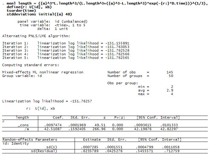
The estimated asymptotic length is 42.5 mm with a standard error of 0.16, and the mean growth rate is 0.0097 with a standard error of 0.0002. The between-lizards standard deviation for the growth rate is 0.0007 with a 95% CI of [0.0005, 0.0011], which suggests that there is variability in lizards’ growth rates compared with their mean value.

Let’s visualize the predicted growth rates for lizards. We can use predict to compute the predictions not only for the response but also for any parameter or function defined in define(). So we use predict to compute lizard-specific and mean growth rates.

Next, we plot the predicted growth rates.

The growth rates of lizards vary around the mean value of 0.0097, with the largest value of 0.0113 for lizard 40 and the smallest value of 0.0083 for lizard 22.

Multiple-dose PK models

PK models concern drug absorption, distribution, metabolism, and excretion. Single-dose and multiple-dose models are of special interest. Each comes in two flavors distinguished by how long it takes the drug to enter the body: orally or intravenously. menl can fit all those models.

Let’s use menl to fit a multiple-dose model with intravenous administration. Consider a study of the neonatal PKs of phenobarbital (Grasela and Donn 1985). Each infant received one or more intravenous doses, dose (mg/kg). One to six blood serum phenobarbital concentration measurements, conc(mg/L), were obtained from each infant, subject. Other variables of interest are birthweight and a dichotomized Apgar score (fapgar), a measure of the physical condition.

A one-compartment open model with intravenous administration and first-order elimination was used to model the PKs of this phenobarbital study.

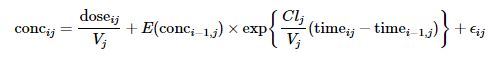
Model parameters are the clearance, $C l_{j}$ (L/h), and volume of distribution, $V_{j}$ (L), for each infant $j$ . $E ({conc}_{i - 1, j})$ is the expected concentration at measurement time $i - 1$ for infant $j$ .

In addition, $C l_{j}$ and $V_{j}$ are parameterized as follows,

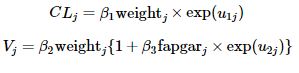
where $u_{1 j}$ and $u_{2 j}$ are two independent Gaussian random effects with zero means and the corresponding variances $σ_{1}^{2}$ and $σ_{2}^{2}$ .

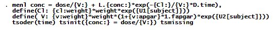
The menl specification is the following.

The explanation of the syntax follows.

Option define() was used to incorporate the parameterizations for $C l_{j}$ and $V_{j}$ . For instance, in option define(Cl:…), {cl:weight} models $β_{1}$ and {U1[subject]} models $u_{1 j}$ .

The difference operator D.time models (time $_{i j} -$ time $_{i - 1, j}$ ).

The expression L.{conc:} models the predicted value for $E ({conc}_{i - 1, j})$ . It represents the predicted value for the concentration corresponding to the previous time value.

Option tsorder(time) specified the variable, time, that will be used to determine the time order for the time-series operators.

Option tsinit() specifies the initial condition for the concentration at time 0.

Option tsmissing specifies that observations containing system missing values (.) in the outcome conc be retained in the computation. In this dataset, these observations represent intermittent measurements at which the dose was administered but the concentration was not measured.

We now fit the model.

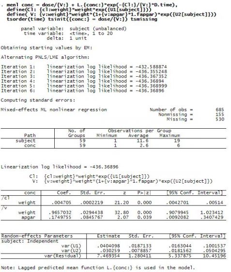
Heavier babies have a higher clearance and volume of distribution. There is a positive association between the volume of distribution and the Apgar score: healthier babies have a better ability to eliminate the drug.

After estimation, let’s use predict to predict concentrations.

The default prediction is the predicted mean function, including the estimates of subject-specific random effects. So variable yhat contains observation-specific mean concentration for each infant.

Let’s plot the predicted concentration against the observed one for, say, the first four infants.

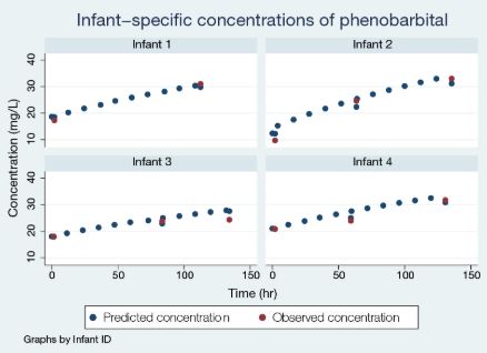
The model predicted the missing intermittent concentrations and provided the entire trajectory of the concentration for the observed measurement times.

Epidemiologia e Biostatistica

Scienze Sociali

Econometria

ECONOMETRIA FINANZIARIA

Corsi per l'utilizzo del software

CONVEGNO ITALIANO DEGLI UTENTI DI STATA

Analisi biostatistica, epidemiologica e ricerca medica

Software per ricerche operative

Analisi statistica generale

formazione multimediale

modelli gerarchici lineari e non lineari

Analisi di data mining

Trasferimento di archivi di dati

Analisi spaziale

Matematica e Ingegneria

word processing scientifico

Analisi statistica specialistica

Disegno di esperimenti e analisi della dimensione dei campioni

Analisi di serie temporali e la stima di modelli econometrici

analisi qualitativa

modelli di reti neurali

STATA PRESS

Altri testi relativi a Stata