Nonparametric tests for trend
Trend tests involve responses in ordered groups. They test whether response values tend to either increase or decrease across groups.
Trend tests are typically used when there is only a small amount of data and no covariates to control for, and a test yielding a p-value valid in small samples is desired. nptrend has an option to compute exact p-values based on Monte Carlo permutations or a full enumeration of the permutation distribution (the latter practical only for extremely small samples).
nptrend performs four different tests for trend:
the Cochran–Armitage test,
the Jonckheere–Terpstra test,
the linear-by-linear trend test, and
a test using ranks developed by Cuzick.
To calculate the Cochran–Armitage statistic for trend, you type
. nptrend relief, group(dose) carmitage
Let’s see it work
For the Cochran–Armitage test (when the response is 0/1), linear-by-linear trend test, and Cuzick’s test, the groups have scores as well. It tests the trend in the proportions of positive responses across the groups.
Here we have fictional data from a clinical trial of a new drug for treating migraines. The variable dose contains the dose of the drug given to a subject. The variable relief is 0/1, with 0 indicating no relief and 1 partial or total relief.
Here is a tabulation of the data:
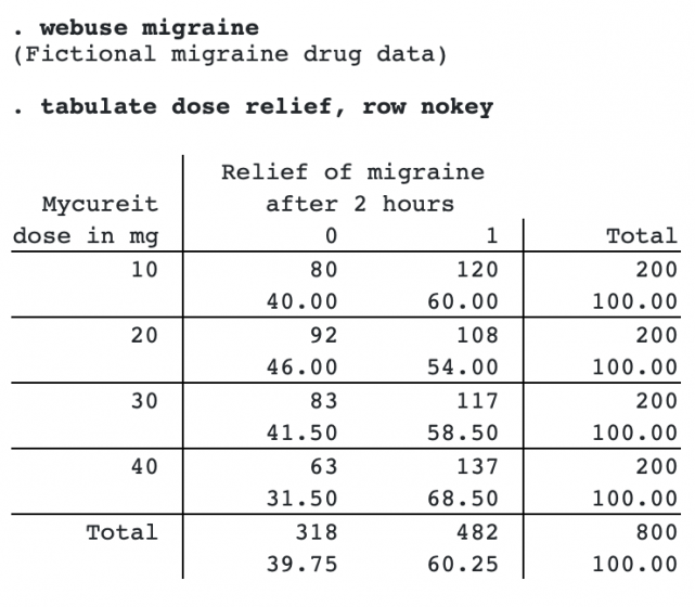
We will test whether there is a trend by dose in the proportion of subjects reporting relief.
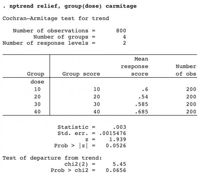
nptrend first displays a table of the mean response score by group. The mean response score in this case is simply the proportion of subjects in the group reporting relief.
The Cochran–Armitage z statistic tests for a linear trend. A χ2 statistic that tests for departure from a linear trend is also calculated.
When either the z statistic for linear trend or the χ2 statistic for departure from linear trend is large, it means that the test for independence between response and group is rejected. z being large means there is a linear trend that rejects independence. χ2 being large means there are differences other than the linear trend that reject independence.
In the example above, the linear test for trend gave a p-value of 0.0526, not quite reaching significance at the 0.05 level. The test of departure from trend gave a p-value of 0.0656, meaning there is weak evidence, not reaching significance, for a nonlinear association between dose and relief.
Trends other than linear can also be tested using the scoregroup() option. For this example, specifying scoregroup(1 4 9 16) would test a quadratic trend in dose.
The Cochran–Armitage test requires that responses be 0/1 or else the group indicator be 0/1. The other trend tests computed by nptrend have no restriction on the response; the response variable can have any value.
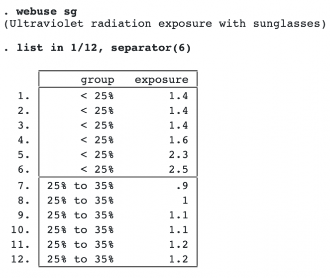
Here’s an example with the responses being ocular exposure to ultraviolet radiation for 32 pairs of sunglasses. Sunglasses are classified into 3 groups according to the amount of visible light transmitted. We list some of the data:
The Jonckheere–Terpstra test is useful when it is not clear what the trend might be and we simply want to test for any trend. It tests whether the ordering of the responses is associated with the ordering of the groups.
To compute the Jonckheere–Terpstra test, we specify the option jterpstra.
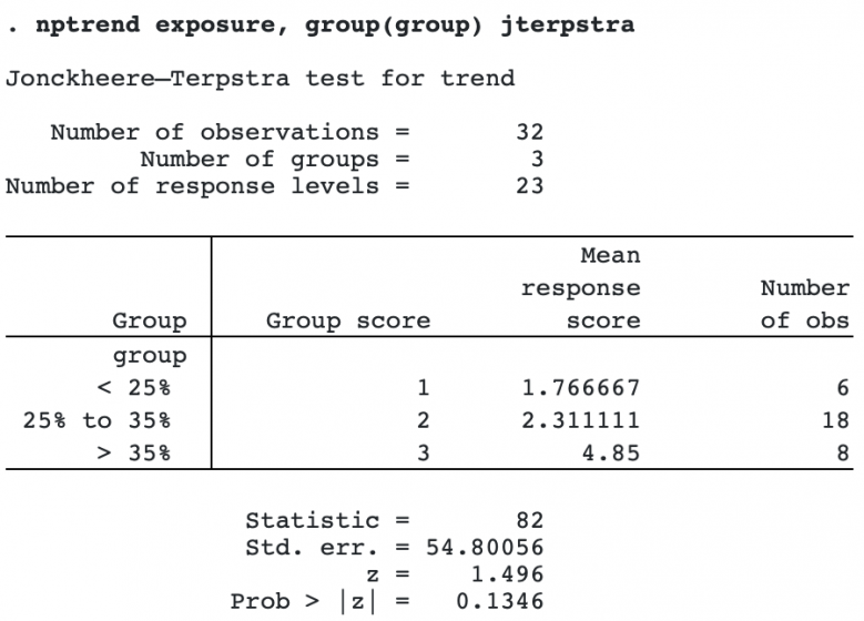
We see that the mean response score increases as the group indicator increases, but the p-value from the Jonckheere–Terpstra test is 0.1346, not reaching significance at the 0.05 level.
Because the Jonckheere–Terpstra statistic tests for any type of trend in responses across ordered groups, it will not be as powerful as a test that accurately hypothesizes the true trend. The linear-by-linear trend test allows you to do just this. The linear-by-linear trend test uses the numeric values of the responses to specify the trend being tested. How the trend is hypothesized to vary across groups is specified by the numeric values of the group variable.
The linear-by-linear statistic is equivalent to the Pearson correlation coefficient, the difference being that the Pearson correlation coefficient is standardized by the standard deviations of the scores. The p-values are slightly different because the p-value for the linear-by-linear test is based on its permutation distribution while the p-value for the Pearson correlation coefficient assumes normality.
To compute the linear-by-linear test, we specify the option linear. We also specify notable to suppress the display of the mean response scores by group.
. nptrend exposure, group(group) linear notable

Linear-by-linear test for trend

   Number of observations =       32
         Number of groups =        3
Number of response levels =       23

                Statistic = .7035156
                Std. err. = .3063377
                        z =    2.297
               Prob > |z| =   0.0216
The p-value from the linear-by-linear test is 0.0216, which is considerably different from the p-value computed by the Jonckheere–Terpstra test, which was 0.1346. This is not surprising because the linear-by-linear test assumes a specific trend based on numerical values, whereas the Jonckheere–Terpstra statistic tests for any trend.
The fourth trend test computed by nptrend is a test based on ranks developed by Cuzick.
. nptrend exposure, group(group) cuzick

. nptrend exposure, group(group) cuzick notable

Cuzick's test with rank scores

   Number of observations =       32
         Number of groups =        3
Number of response levels =       23

                Statistic =  1.65625
                Std. err. = 1.090461
                        z =    1.519
               Prob > |z| =   0.1288
In this case, it produces a p-value that is similar to the p-value from the Jonckheere–Terpstra test.
Exact p-values
nptrend will also compute exact p-values using Monte Carlo permutations when the exact option is specified. Here we compute the exact p-value for the Jonckheere–Terpstra test.
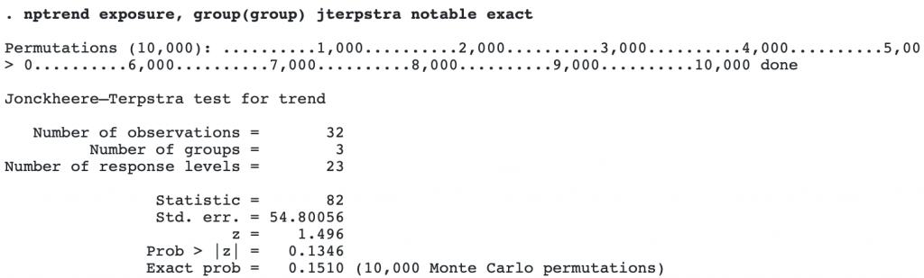
By default, 10,000 Monte Carlo permutations are used. This gave an exact p-value of 0.1510, differently slightly from the p-value of 0.1346, computed using a normal approximation.
Monte Carlo permutations give results with random error, so for more precision, more permutations can be computed. Below, we use 100,000 permutations, and have a dot displayed every 1,000th permutation to monitor the progress. We specify a random-number seed so we can duplicate the results and the option show, which displays a detailed table of the Monte Carlo results.
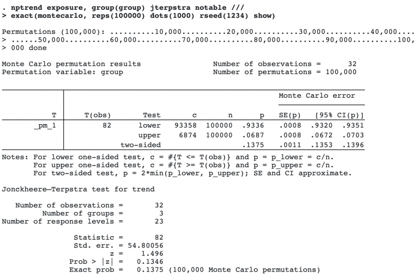
The exact p-value from the Monte Carlo computation is 0.1375, close to the approximate p-value of 0.1346. From the detailed table of the results, we see that the 95% confidence interval for the Monte Carlo p-value is [0.1353, 0.1396], which does not include the approximate p-value.
This example has only 32 observations. Should we wish to publish the results, we would likely want to run nptrend again, specifying 1,000,000 or more permutations to reduce the Monte Carlo error further. Permutations are generated using a fast algorithm, and the computation is not time-consuming.
For extremely small datasets, the exact(enumerate) option can be used to fully enumerate the permutation distribution. It gives an exact p-value without any Monte Carlo error.