Stata fits multilevel mixed-effects generalized linear models (GLMs) with meglm. GLMs for cross-sectional data have been a workhorse of statistics because of their flexibility and ease of use. Stata’s xtgeecommand extends GLMs to the use of longitudinal/panel data by the method of generalized estimating equations.
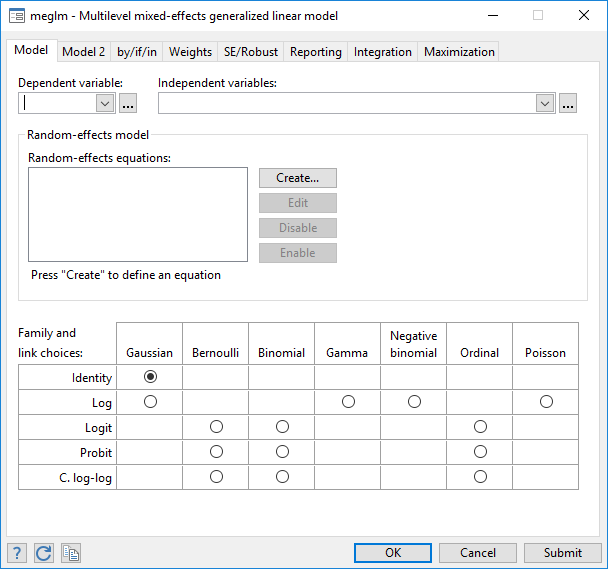
Now you can use meglm to fit GLMs to hierarchical multilevel datasets with normally distributed random effects. Seven distributions for the response variable are supported (Gaussian, Bernoulli, binomial, gamma, negative binomial, ordinal, and Poisson); and five link functions are possible (identity, log, logit, probit, and complementary log-log).
Let’s fit a three-level model.
We have student-level data, where students are nested in classes, and classes are nested in schools. Our dependent variable thk is an ordered categorical variable that takes on the values 1, 2, 3, or 4; and we have three explanatory variables: prethk, cc, and tv. We will treat prethk as continuous. cc and tv are binary, and we want to include their interaction the model. Let’s fit an ordered logit model:
. webuse tvsfpors
. meglm thk prethk cc##tv || school: || class:, family(ordinal) link(logit)
Fitting fixed-effects model:
Iteration 0: log likelihood = -2212.775
Iteration 1: log likelihood = -2125.509
Iteration 2: log likelihood = -2125.1034
Iteration 3: log likelihood = -2125.1032
Refining starting values:
Grid node 0: log likelihood = -2152.1514
Fitting full model:
Iteration 0: log likelihood = -2152.1514 (not concave)
Iteration 1: log likelihood = -2125.9213 (not concave)
Iteration 2: log likelihood = -2120.1861
Iteration 3: log likelihood = -2115.6177
Iteration 4: log likelihood = -2114.5896
Iteration 5: log likelihood = -2114.5881
Iteration 6: log likelihood = -2114.5881
Mixed-effects GLM Number of obs = 1,600
Family: ordinal
Link: logit
| Group Variable | No. of Groups | Observations per Group Minimum | Observations per Group Average | Observations per Group Maximum |
| school | 28 | 18 | 57.1 | 137 |
| class | 135 | 1 | 11.9 | 28 |
Integration method: mvaghermite Integration points = 7
Wald chi2(4) = 124.39
Log likelihood = -2114.5881 Prob > chi2 = 0.0000
| thk | Coef. | Std. Err. | z | P>|z| | [95% Conf. Interval] | [95% Conf. Interval] |
| prethk | .4085273 | .039616 | 10.31 | 0.000 | .3308814 | .4861731 |
| 1.cc | .8844369 | .2099124 | 4.21 | 0.000 | .4730161 | 1.295858 |
| 1.tv | .236448 | .2049065 | 1.15 | 0.249 | -.1651614 | .6380575 |
| cc#tv
1 1 |
-.3717699 | .2958887 | -1.26 | 0.209 | -.951701 | .2081612 |
| /cut1 | -.0959459 | .1688988 | -0.57 | 0.570 | -.4269815 | .2350896 |
| /cut2 | 1.177478 | .1704946 | 6.91 | 0.000 | .8433151 | 1.511642 |
| /cut3 | 2.383672 | .1786736 | 13.34 | 0.000 | 2.033478 | 2.733865 |
| school
var (_cons) |
.0448735 | .0425387 | .0069997 | .2876749 | ||
| school>class
var (_cons) |
.1482157 | .0637521 | .063792 | .3443674 |
LR test vs. ologit regression: chi2(2) = 21.03 Prob > chi2 = 0.0000
Note: LR test is conservative and provided only for reference.
Our model has two random-effects equations, separated by ||. Our first is a random intercept at the school level, and the second is a random intercept at the class level. The order we listed them matters: class comes after school, meaning that classes are nested within schools. Using the same logic, we could include more levels of nesting. meglm also allows crossed-effects models.
The output table includes the fixed-effect portion of our model, the estimated cutpoints (because this is an ordered logit model), and the estimated variance components.
This model can alternatively be fit with meologit, which is a convenient use for meglm with an ordinal family and a logit link.