Zero-inflated ordered logit model

Stata’s new ziologit command fits zero-inflated ordered logit models.

Ordered logit regression is used to model ordered categorical responses, such as symptom severity recorded as none, mild, moderate, or severe. Larger values of such ordered outcomes represent higher levels, but the numeric value is irrelevant.

In some situations, more zeros (or more values in the lowest category) are observed in the data than would be expected by a traditional ordered logit model. A zero might represent the absence of a trait, while the remaining values represent increasing levels of the trait. Many zeros may be observed, some because the individual does not have the trait and some because an individual has the trait but exhibits the lowest level. For example:

In a study of alcohol consumption, some individuals report no consumption because they never drink alcohol, while others may report no alcohol consumption because they did not drink in the survey period.

In a clinical trial of a treatment intended to shrink tumors, outcomes represent no improvement, partial response, or complete response. An individual may show no improvement because the tumor is resistant to treatment or because the tumor was treatable but did not shrink at the time of measurement. The distinction is important because treatable tumors are good candidates for a higher dose.

In contexts such as these, you can use a zero-inflated ordered logit (ZIOL) model. ZIOL models assume that the lowest-valued outcomes come from both a logit model and an ordered logit model, allowing different sets of predictors for each model.

Let’s see it work

Let’s use fictional data on daily cigarette consumption. The codebook command shows us the four levels of cigarette consumption.

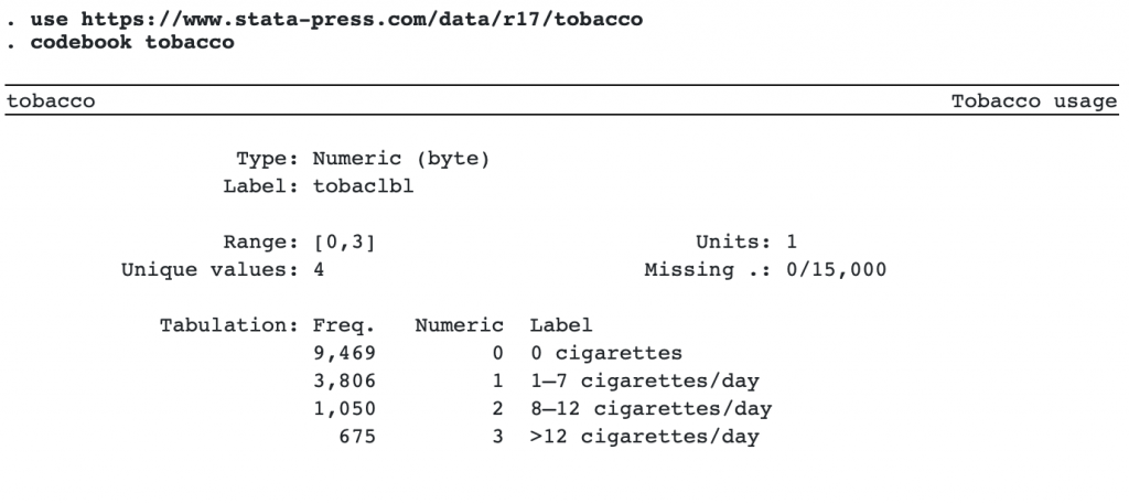
More than half the respondents reported zero cigarette consumption. A zero may be reported for two reasons—because a respondent is always a nonsmoker or because a respondent is susceptible to smoking but did not smoke in the time period for which the data were collected. A traditional ordered logit model cannot distinguish between the two causes of zero cigarette consumption. The ZIOL model allows us to model the probability of being susceptible to smoking in addition to modeling level of consumption.

We fit the ZIOL model by using ziologit. We model the level of cigarette consumption as a function of education (education), income in $10,000s (income), and gender (female). We specify the inflate() option to model the probability of being a smoker as a function of education, income, and whether the respondent’s parents smoked (parent).

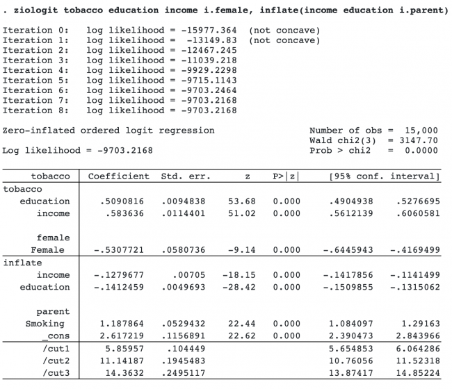
The first section of the table, labeled “tobacco”, reports results for the ordered logit model of cigarette consumption. The second section, labeled “inflate”, reports results for the logit model of the probability of being a smoker.

To more easily interpret the results from the first two sections, we request that ziologit show odds ratios rather than coefficients.

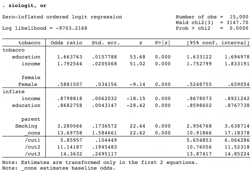
A $10,000 increase in annual income decreases the odds of being a smoker by a factor of 0.88 (12% decrease in odds) but, among smokers, increases the odds of higher cigarette consumption by a factor of 1.79 (79% increase in odds). This suggests that wealthier individuals are less likely to smoke, but if they do decide to smoke, they tend to smoke more cigarettes.

But what do these results mean in terms of the probability of exhibiting different smoking behavior? Suppose we want to know the relationship of cigarette consumption to income level. For that, we use the margins command. For annual incomes of $0, $50,000, $100,000, $150,00, and $200,000, we estimate the expected probabilities of each cigarette consumption level.

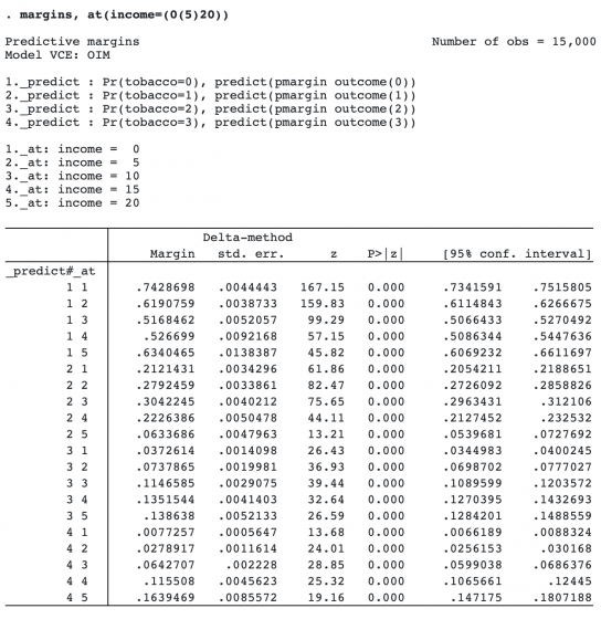
We estimated many expected probabilities. It is helpful to visualize the results by using marginsplot.

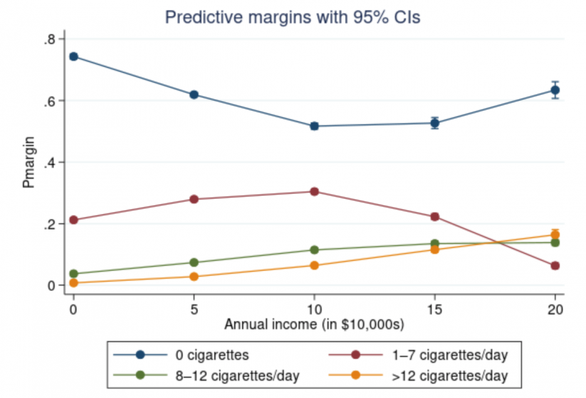
The probability of smoking 0 cigarettes decreases as annual income increases until $100,000; then, the probability gradually increases again. The probability of smoking 1–7 cigarettes/day is highest when earnings are $100,000 per year, and lowest when earnings are $200,000 per year.

We now want to examine the relationship between income and the susceptibility to smoking. We add the predict(ps) option to margins to request the estimates of predicted probability of susceptibility.

. quietly margins, predict(ps) at(income=(0(5)20))

. marginsplot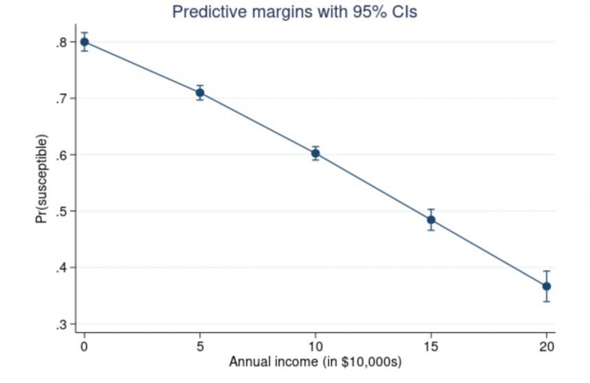

Four-fifths of respondents when income is zero are susceptible to smoking. The probability of being a smoker decreases with increasing income, with just over a third of respondents susceptible to smoking when earnings are $200,000 per year. This supports the interpretation that income may act as a proxy for health consciousness.

Next we use margins to focus on subjects who are susceptible to smoking. By specifying statistic pcond1 along with each outcome level, we calculate the probability of each level of tobacco, conditional on susceptibility. As before, calculations are performed at five levels of income and graphed with marginsplot.

. quietly margins, predict(pcond1 outcome(0)) predict(pcond1 outcome(1))
 predict(pcond1 outcome(2)) predict(pcond1 outcome(3)) at(income=(0(5)20))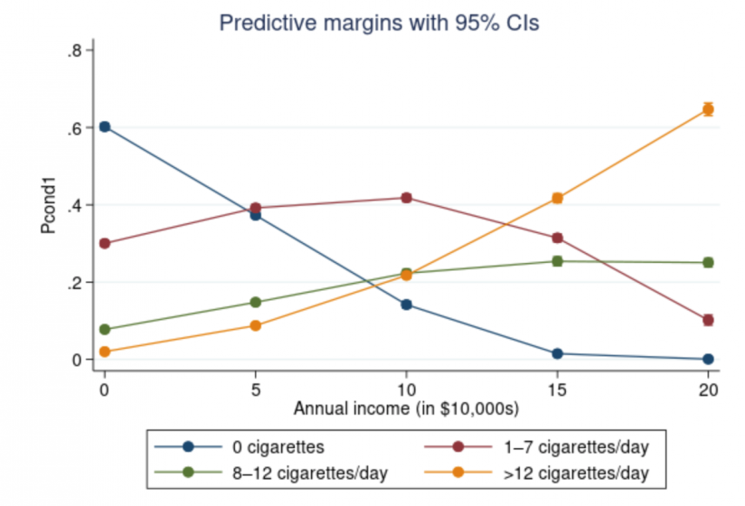

When annual income is zero, well over half of those susceptible to smoking report zero cigarette consumption, and those who do consume cigarettes are most likely to smoke just a few cigarettes per day. As income increases, the probability of zero consumption falls. Higher annual income is associated with a higher probability of being a heavy smoker. This suggests that, among smokers, cigarettes are treated as what economists call a normal good, that is, something for which demand increases when income increases.

We can see from this example that the effect of income on cigarette consumption is multifaceted. The ziologit command makes it possible to model smoking susceptibility as well as smoking intensity, leading to a better understanding of the factors influencing smoking behavior.