THE GS SUITE
The gs suite provides two commands: gsbounds and gsdesign.
The gsbounds command calculates efficacy and futility bounds based on the number of analyses, also called looks, the desired overall type I error, and the desired power.
You can select from seven boundary-calculation methods:
- Classical O’Brien–Fleming
- Classical Pocock
- Classical Wang–Tsiatis
- Error-spending Pocock style
- Error-spending O’Brien–Fleming style
- Error-spending Kim–DeMets
- Error-spending Hwang–Shih–de Cani
To calculate, for instance, O’Brien–Fleming efficacy and futility bounds for a study with 5 looks, a power of 0.9, and a type I error of 0.05, type
. gsbounds, efficacy(obfleming) futility(obfleming) nlooks(5)
  power(0.9) alpha(0.05)
Want to visualize these boundaries? Add the graphbounds option to the above command.
The gsdesign command computes efficacy and futility boundaries and provides sample sizes at each look for a variety of tests. gsdesign is specified with one of the subcommands listed below, depending on the type of test to be performed for the trial.
| Command | Description |
|---|---|
|
gsdesign onemean |
GSD for a one-sample mean test |
|
gsdesign twomeans |
GSD for a two-sample means test |
|
gsdesign oneproportion |
GSD for a one-sample proportion test |
|
gsdesign twoproportions |
GSD for a two-sample proportions test |
|
gsdesign logrank |
GSD for a log-rank test |
|
gsdesign usermethod |
GSD for a user-defined method |
THE GS SUITE IN ACTION!
Suppose we are interested in designing a group sequential trial for a new pediatric COVID-19 vaccine (our experimental treatment), which we will compare against the first-generation vaccine (our control treatment). We will measure the log of participants’ neutralizing antibody titers and compare the mean log-titer in the experimental group with that of the control group. We can use gsdesign twomeans to calculate stopping boundaries and required sample sizes for such a trial.
Say that we anticipate a mean log-titer of 5.5 with known standard deviation of 2 in the control arm and a mean log-titer of 6.5 with known standard deviation of 3 in the experimental arm. We will compute sample sizes for a one-sided test at the 2.5% level with power of 90% and will allocate twice as many participants to the experimental arm as to the control arm.
We calculate sample sizes for five looks (four interim analyses and a final analysis), scheduled to occur with 50%, 65%, 80%, 90%, and 100% of the data. We calculate efficacy and nonbinding futility boundaries using the error-spending approximation of classical O’Brien–Fleming boundaries.
© Copyright 1996–2024 StataCorp LLC. All rights reserved.
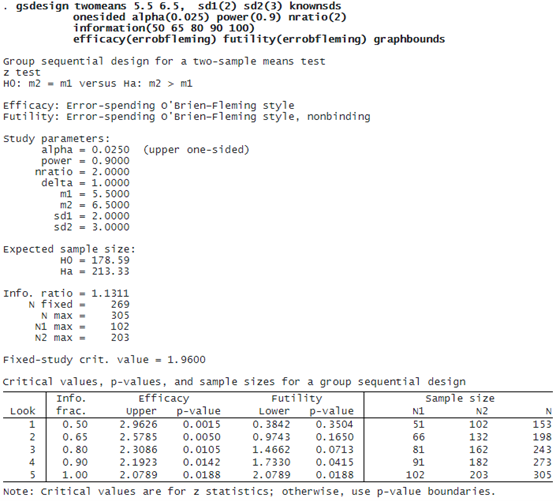
If this trial continues to the final analysis, 305 participants will be required. However, the expected sample size is smaller—179 if the null hypothesis is true and 213 if the alternative hypothesis is true. An equivalent fixed study design, which does not have the option to stop early, would require 269 participants.
The table at the bottom of the output presents the stopping boundaries as both critical z-values and p-values, as well as the sample size required at each analysis. The first look occurs once data are collected from 51 participants in the control arm and 102 participants in the experimental arm. If the z statistic is greater than or equal to 2.96, then H0 is rejected and the trial is stopped. If the z statistic is less than 0.38, then H0 can be accepted, and the trial can be terminated for futility. However, because the futility boundary is nonbinding, even if the z statistic is less than 0.38, the trial is allowed to continue without overrunning the familywise type I error. If the z statistic at the first look is between 0.38 and 2.96, the trial must continue collecting data until the second look.
The testing procedure at the second, third, and fourth looks is akin to that of the first look; the difference is that the efficacy and futility bounds get progressively closer. At the fifth and final look, which takes place once data have been collected from 102 participants in the control arm and 203 participants in the experimental arm, the efficacy critical value equals the futility critical value, and there is no option to continue. If the z statistic at the final look is greater than or equal to 2.08, then H0 is rejected; otherwise, H0 is accepted.
The graph produced when the graphbounds option is specified makes it easy to visualize the stopping boundaries and the required actions to be taken at each look.

When a z statistic falls within the blue rejection region, the trial is stopped for efficacy. When the z statistic falls within the red acceptance region, the trial can be stopped for futility. If the z statistic falls in the green continuation region, the trial continues to the next look.