Bayesian VAR models
Vector autoregressive (VAR) models study relationships between multiple time series, such as unemployment and inflation rates, by including lags of outcome variables as model predictors. That is, the current unemployment rate would be modeled using unemployment and inflation rates at previous times. And likewise for the current inflation rate.
VAR models are known to have many parameters: with K outcome variables and p lags, there are at least K(pK+1) parameters. Reliable estimation of the model parameters can be challenging, especially with small datasets.
You can use the new bayes: var command to fit Bayesian VAR models that help overcome these challenges by incorporating prior information about model parameters. This often stabilizes parameter estimation. (Think of a prior as introducing a certain amount of shrinkage for model parameters.)
You can investigate the influence of a random-walk assumption on the results by varying the parameters of several supported variations of the original Minnesota prior distribution. You can check the assumption of a parameter stability by using the new command bayesvarstable. Once satisfied, you can generate dynamic forecasts by using bayesfcast and perform impulse–response function (IRF) and forecast-error variance decomposition (FEVD) analysis by using bayesirf.
Let’s see it work
Estimation
Checking parameter stability
Customizing the default prior
Selecting the number of lags
IRF analysis
Dynamic forecasts
Clean up
Estimation
Consider Federal Reserve quarterly economic macrodata from the first quarter of 1954 to the fourth quarter of 2010. We would like to study the relationship between inflation, the output gap, and the federal funds rate. We wish to evaluate how each of these macroeconomic variables affects the others over time. In particular, we are interested in the effects of the federal fund rate controlled by policymakers. We are also interested in obtaining dynamic forecasts for the three outcome variables.
Let’s take a look at our data first.
. webuse usmacro
(Federal Reserve Economic Data - St. Louis Fed)

. tsset

Time variable: date, 1954q3 to 2010q4
        Delta: 1 quarter

. tsline inflation ogap fedfunds

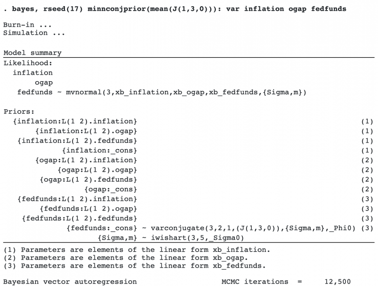
We wish to fit a Bayesian VAR model to study the relationship between the three variables. If you are already familiar with Stata’s var command, which fits classical VAR models, fitting Bayesian models will be particularly easy. We simply prefix the var command with bayes:. Below, we also specify a random-number seed for reproducibility.
The output from bayes: var is long, so we will describe it in pieces.
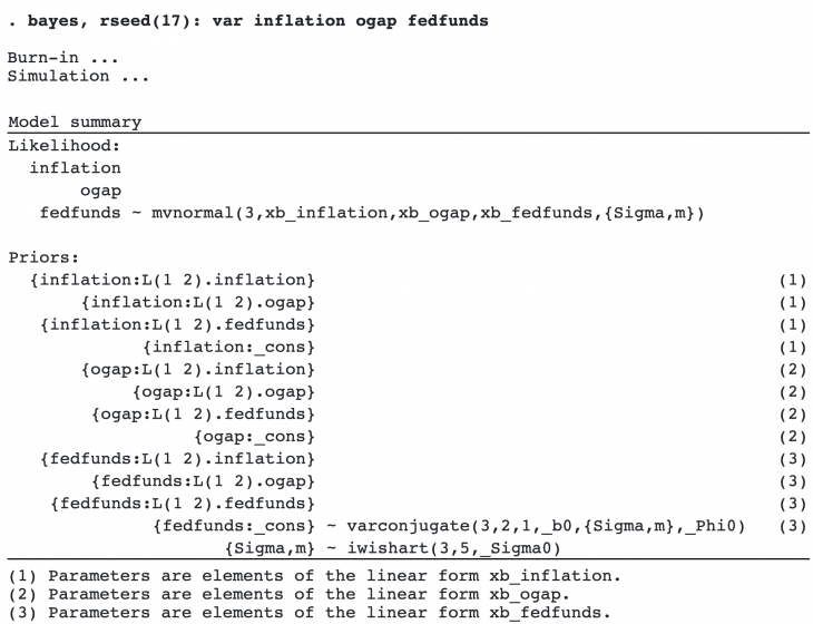
As with a traditional VAR model, the likelihood is assumed to be multivariate (trivariate in our example) normal with the error covariance matrix{Sigma,m}. The error covariance is a model parameter, so it appears in curly braces, {}.
A Bayesian VAR model additionally requires priors for all model parameters. bayes: var provides default priors, but you can modify them to adjust to your analysis.
By default, VAR regression coefficients are assigned a so-called conjugate Minnesota prior, and the error covariance is assigned an inverse Wishart prior. The idea behind a Minnesota prior is to “shrink” coefficients toward some values (often zeros or ones for the first own-lag coefficients) while maintaining the underlying time-dependent relationships in the data. You can learn more about this prior in Explaining the Minnesota prior in [BAYES] bayes: var.
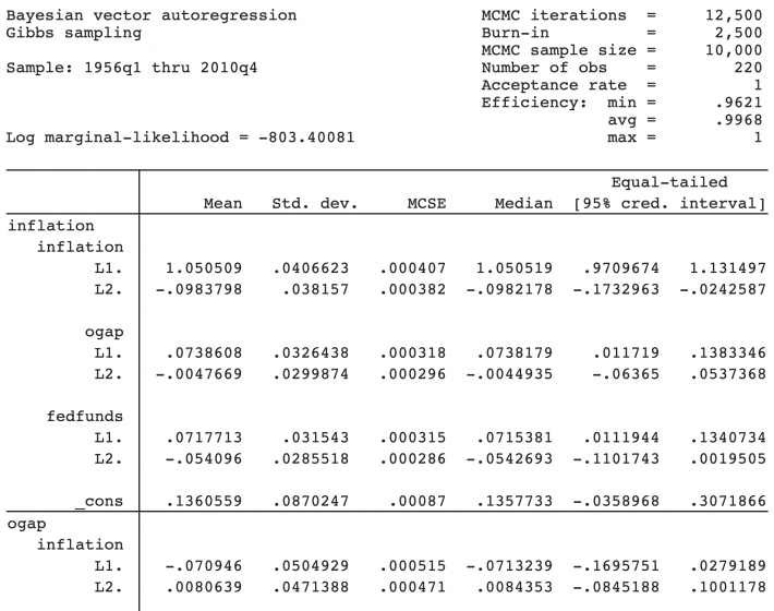
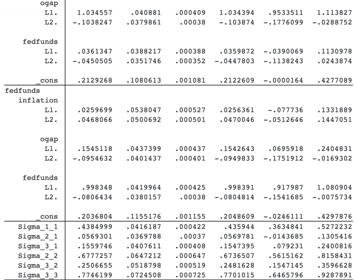
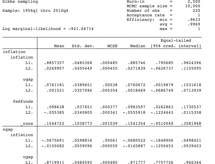
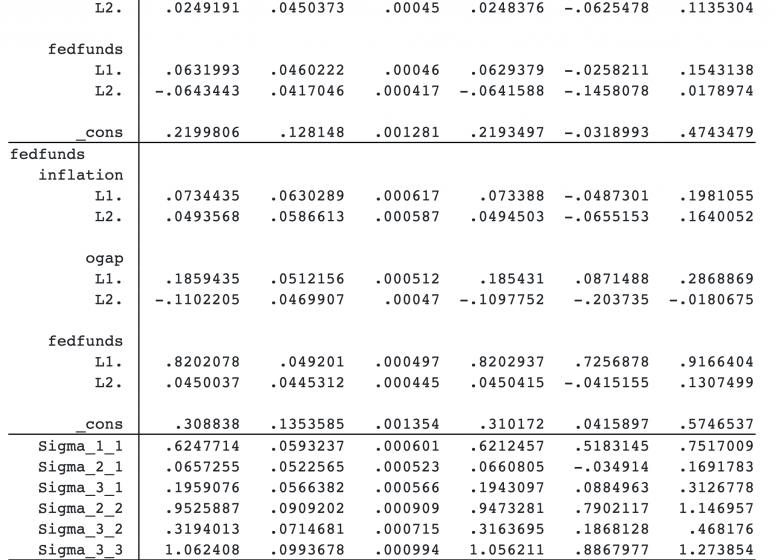
What follows next is a rather lengthy output of results. As we will see in IRF analysis, the results from a VAR model are usually interpreted by using IRFs and other functions. But we show the output below for completeness.
The header reports the standard information about the MCMC procedure: the number of burn-in iterations, the size of the MCMC sample, and so on. The defaults are 2,500 burn-in iterations and 10,000 for the MCMC sample size, but you may need fewer or more in your analysis. Because bayes: var uses Gibbs sampling for simulation, the MCMC results will typically have high efficiency (close to 1); see the output below under Efficiency:
By default, bayes: var includes two lags for each outcome variable, but you can specify other lags in the lags() option; see Selecting the number of lags.
After simulation, you may want to save your MCMC results for further postestimation analysis. With bayes, this can be done either during or after estimation.
. bayes, saving(bvarsim2)
note: file bvarsim2.dta saved.
We also store the current bayes: var estimation results for later model comparison.
. estimates store lag2
As with any MCMC method, we should check that MCMC converged before moving on to other analyses. We can use graphical checks,
. bayesgraph diagnostics {inflation:L1.ogap}

or we can compute the Gelman–Rubin convergence statistic using multiple chains. The trace plot does not exhibit any trend, and the autocorrelation is low. Our MCMC appears to have converged.
Checking parameter stability
Inference from a VAR model relies on the assumption of parameter stability, which you can check after a Bayesian VAR model by using the new command bayesvarstable.
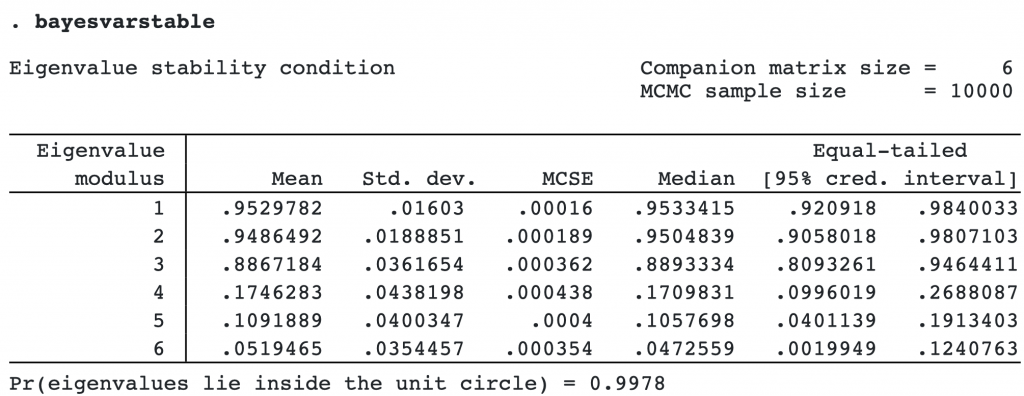
The 95% credible intervals for individual eigenvalue moduli do not contain values greater or equal to one, which is a good sign. And the posterior probability that all eigenvalues lie in the unit circle is close to one. We have no reason to suspect a violation of the stability assumption.
Customizing the default prior
By default, the conjugate Minnesota prior of bayes: var shrinks the first own-lag coefficients toward one. (A first own-lag coefficient is a coefficient for the first lag of the outcome variable in its own equation. In our example, there are three such coefficients: {inflation:L1.inflation}, {ogap:L1.ogap}, and{fedfunds:L1.fedfunds}.)
The default prior favors the assumption of a random walk for the outcome variable. This assumption may or may not be what you want depending on the data type. For instance, with differenced data, you may want to shrink all of the coefficients toward zero.
We can do this by modifying the default specification of the minnconjugate() option, which specifies the conjugate Minnesota prior. The default prior assumes prior means of ones only for the first own-lag coefficients. Prior means of the other coefficients are already zeros. So we need to specify zero means only for the three first own-lag coefficients. We can do this by specifying a vector of length 3 of 0s in minnconjprior()‘s suboption mean().
The new prior specification did not appear to change the results much. This means that the information contained in the observed data about the model parameters dominates our prior information.
Selecting the number of lags
A lag selection is an important consideration for VAR models. Traditional methods, such as those using the AIC criterion, often overestimate the number of lags. Bayesian analysis allows you to compute an actual probability of each model given the observed data—model posterior probability.
To compute model posterior probabilities, we must first fit all the models of interest. Let’s consider one, two, and three lags here, but you can specify as many models as you would like in your own analysis.
We already stored the results from the model with two lags as lag2. We now fit models with one and three lags and save the corresponding results. We run the models quietly.
. quietly bayes, rseed(17) saving(bvarsim1): var inflation ogap fedfunds, lags(1/1)
. estimates store lag1

. quietly bayes, rseed(17) saving(bvarsim3): var inflation ogap fedfunds, lags(1/3)
. estimates store lag3
We now use bayestest model to compute model posterior probabilities. We assume that each model is equally likely a priori (the default).
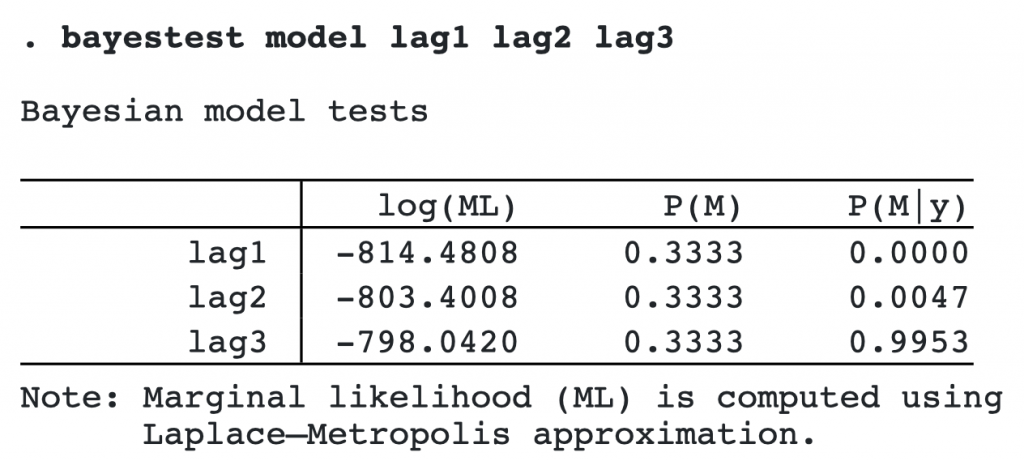
The model with three lags has the highest posterior probability of the three considered models.
IRF analysis
VAR models contain many regression coefficients, which makes it difficult to interpret the results from these models. Instead of individual coefficients, IRFs are used to summarize the results. IRFs measure the effect of a shock in one variable, an impulse variable, on a given response variable at a specific time period.
In our example, we are interested in the impact of the federal funds rate on the other outcomes in the model. Let’s use IRFs to evaluate the effect of this variable.
Here we use the model with three lags that we selected in the previous section.
. estimates restore lag3
(results lag3 are active now)
As with a standard IRF analysis in Stata, we first create IRF results and save them in an IRF dataset for later analysis. For IRF analysis after bayes: var, we use the new bayesirf command instead of the existing irf command.
The new command is needed because of the differences between classical and Bayesian IRFs. For a given pair of impulse and response variables, a frequentist IRF is a single function, whereas Bayesian IRFs correspond to a posterior MCMC sample of functions. This sample is summarized to produce a single function. The posterior mean IRF is reported by default, but you can compute the posterior median IRF instead.
First, we use bayesirf create to create IRF results named birf and save them in the IRF file birfex.irf.
. bayesirf create birf, set(birfex)
(file birfex.irf created)
(file birfex.irf now active)
(file birfex.irf updated)
We plot IRFs with fedfunds as the impulse variable.
. bayesirf graph irf, impulse(fedfunds)

This IRF graph shows that a shock to the federal funds rate has a positive effect on itself that decreases over time but is still positive after 8 quarters. The federal funds rate shock has little effect on the output gap and a small positive effect on inflation that dissipates after 2 quarters.
Also see Bayesian IRF and FEVD analysis.
Dynamic forecasts
VAR models are commonly used for forecasting. Here we show how to compute Bayesian dynamic forecasts after fitting a Bayesian VAR model.
We create forecasts after bayes: var just as we do after var, except we use bayesfcast instead of fcast.
Similarly to Bayesian IRFs, Bayesian forecasts correspond to the posterior MCMC sample of forecasts for each time period. The posterior mean forecast is reported by default, but you can compute the posterior median forecast instead.
Let’s compute a Bayesian dynamic forecast at 10 time periods.
. bayesfcast compute f_, step(10)
The posterior mean forecasts, together with other forecast variables, are saved in the dataset in variables with outcome names prefixed with f_.
We can use bayesfcast graph to plot the computed forecasts.
. bayesfcast graph f_inflation f_ogap f_fedfunds

From this graph, our inflation forecast is small for the first quarter but is not statistically significant after that. (The 95% credible bands include zero.) The forecasted output gap is negative for the first year and is close to zero after that. The federal funds rate is forecasted to be small and close to zero for all periods.
Also see Bayesian dynamic forecasting.
Clean up
After your analysis, remember to remove the datasets generated by bayes: var and bayesirf, which you no longer need.
. erase bvarsim1.dta
. erase bvarsim2.dta
. erase bvarsim3.dta
. erase birfex.irf