GOALS
Today we will look at the GAUSS kalman filter procedure, which is included in the TSMT application module.
In this tutorial we will use an AR(2) example to examine
- State space representation
- How to define system matrices
- How to use the GAUSS
kalmanFilterprocedure - How to interpret the results of the
kalmanResultstructure.
INTRODUCTION
The Kalman filter is a tool that allows us to determine the optimal estimates of an unobserved state vector, αt, using the observed information at time t.
Today will demonstrate the use of the Kalman filter to predict an AR(2) model from simulated data. We generate our sample AR(2) model using the data generating process
![]()
STATE SPACE REPRESENTATION
The GAUSS kalmanFilter procedure requires that models take a state space representation. Therefore, we must understand how to translate our problem into proper state space representation.
State space representation is composed of three pieces:
- An observation equation.
- A measurement equation.
- An initial state distributions.
The observation equation represents an observed time-series vector
![]()
The transition equation represents an unobserved state vector
![]()
Finally, the initial state distribution represents starting values of the state vector. It includes the initial prior state mean, α0, and the initial prior state covariance, P0.
![]()
STATE SPACE REPRESENTATION OF AN AR(2) MODEL
Putting models into state space representation is somewhat of an art form and there can be many different representations of the same model.
Let’s consider putting a general AR(2) model into the state space representation starting from the standard representation
![]()
AR(2) REPRESENTATION #1
For our first representation we will define
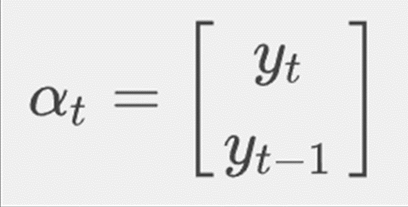 then our measurement equation becomes
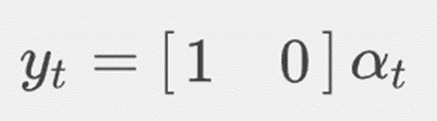
and our transition equation becomes
![]()
To see how this works, let’s look more closely at the matrix multiplication. Consider first plugging αt into our measurement equation
![]()
and
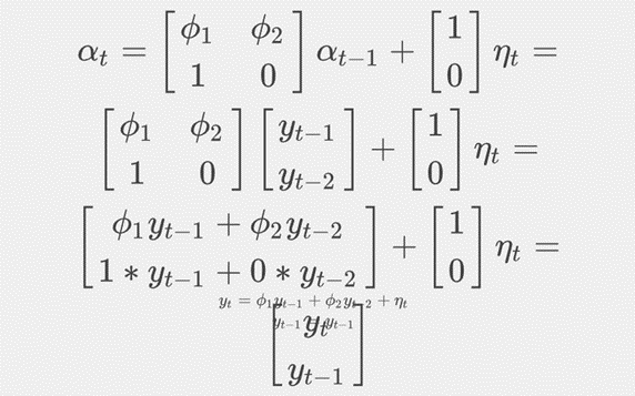
which simplifies to
![]()
AR(2) REPRESENTATION #2
We could also an alternative representation where we let
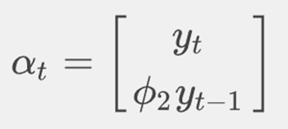
then our measurement equation becomes
![]()
and our transition equation becomes
![]()
USING THE GAUSS KALMAN FILTER
The GAUSS kalmanFilter procedure takes 10 inputs. The first of these inputs is the observed data, yt. We will use the TSMT application module procedure simarmamt to generate our data.
OBSERVED AR(2) DATA
library tsmt;
// Simulate AR(2) data
 seed = 527453;
// Intercept
 b = 0.3|-0.6;
// AR terms
 p = 2;
// MA terms
 q = 0;
// Constant
 const = 0;
// Trend
 trend = 0;
// Number of observations
 n = 150;
// Number of replications
 k = 1;
// Standard deviation of error process
 std = 1;
// Generate data
 y = simarmamt(b, p, q, const, trend, n, k, std, seed)';
SYSTEM MATRICES
The 2nd through 8th inputs into the kalmanFilter procedure are based on the system matrices of the general state space representation.
| GAUSS kalmanFilter system matrices inputs | |
| Z<\td> | The design matrix. |
| d<\td> | The measurement equation intercept. |
| H<\td> | The measurement equation disturbance covariance matrix. |
| T<\td> | The transition matrix. |
| c<\td> | The state transition equation intercept. |
| R<\td> | The selection matrix. |
| Q<\td> | The state disturbance covariance matrix. |
© 2026 Aptech Systems, Inc. All rights reserved.
 /*
 ** Use the two true
 ** phi values
 */
 phi = 0.3|-0.6;
// State disturbance sigma
 sigma2_q = 1;
// Observation disturbance sigma
 sigma2_h = 1;
// Design matrix
 Z = {1 0};
// Measurement equation intercept
 d = 0;
// Measurement equation disturbance
 H = sigma2_h;
// Transition matrix
 T = {phi[1] phi[2], 1 0};
// Transition equation intercept
 c = 0;
// Transition equation disturbance
 Q = sigma2_q;
// Selection matrix
 R = {1, 0};
INITIAL STATE DISTRIBUTION
Before we can run the Kalman filter we must initialize the state vector. This requires specifying both α0, the initial prior state mean, and P0, the initial prior state covariance.
// Initial state mean
 a_0 = 0|0;

// Initial state covariance
 P_0 = {1 0, 0 1};
CALLING THE KALMANFILTER PROCEDURE
The kalmanFilter returns output to a kalmanResult structure whose members will be discussed in the next section. The important thing to note now is that before calling the procedure we must declare an instance of the kalmanResult structure.
struct kalmanResult rslt;
 rslt = kalmanFilter(yt, Z, d, H, T, c, R, Q, a_0, p_0);
SUMMARY OF HOW TO USE KALMANFILTER
We have covered a lot of information in this section. It may be helpful to have a summary of the steps we have to take to use the kalmanFilter procedure:
- Determine state space representation.
- Define the observed data vector.
- Define the system matrices.
- Define the initial state mean and initial state covariance.
- Declare the
kalmanResultstructure and call thekalmanFilterprocedure.
THE kalmanResult STRUCTURE
All output from the kalmanFilter procedure is stored in the kalmanResult structure. The members of the kalmanResult instance kout include:
| kout.filtered_state | The filtered states. |
| kout.filtered_state_cov | Filtered state covariances. |
| kout.predicted_state | The predicted states. |
| kout.predicted_state_cov | Predicted state covariances. |
| kout.forecast | Forecasts. |
| kout.forecast_error | Forecast error. |
| kout.forecast_error_cov | Forecast error covariances. |
| kout.loglikelihood | Computed log likelihood. |
Let’s plot the results stored in kout.predicted_state against a scatter plot of the original data (view the code to produce the graphs here).

We can see that the predicted state closely follows our observed data.
CONCLUSION
Congratulations! You have completed the Kalman filter tutorial. In this tutorial, we used an AR(2) example to examine
- State space representation
- How to define system matrices
- How to use the GAUSS
kalmanFilterprocedure - The members of the
kalmanResultstructure.
For your convenience, the entire code is available below.
 library tsmt;
// Simulate AR(2) data
 seed = 527453;
// Intercept
 b = 0.3|-0.6;
// AR terms
 p = 2;
// MA terms
 q = 0;
// Constant
 const = 0;
// Trend
 trend = 0;
// Number of observations
 n = 150;
// Number of replications
 k = 1;
// Standard deviation of error process
 std = 1;
// Generate data
 y = simarmamt(b, p, q, const, trend, n, k, std, seed)';
/*
 ** Use the two true
 ** phi values
 */
 phi = 0.3|-0.6;
// State disturbance sigma
 sigma2_q = 1;
// Observation disturbance sigma
 sigma2_h = 1;
// Design matrix
 Z = {1 0};
// Measurement equation intercept
 d = 0;
// Measurement equation disturbance
 H = sigma2_h;
// Transition matrix
 T = {phi[1] phi[2], 1 0};
// Transition equation intercept
 c = 0;
// Transition equation disturbance
 Q = sigma2_q;
// Selection matrix
 R = {1, 0};
// Initial state mean
 a_0 = 0|0;
// Initial state covariance
 P_0 = {1 0, 0 1};
struct kalmanResult rslt;
 rslt = kalmanFilter(yt, Z, d, H, T, c, R, Q, a_0, p_0);