INTRODUCTION
Suppose we have stationary univariate time series data but are uncertain about the order of the regressive relationship. You may wish to first use the sample autocorrelation function to help identify the general structure of the model. This can be achieved in GAUSS using the acf functions.
SAMPLE AUTOCORRELATIONS
The acf function computes the sample autocorrelations for a single series. The function internally demeans the series, so there is no need to demean data before calling acf.
The acf function requires the following three inputs:
y
N x 1 data matrix.
k
Scalar denoting the maximum number of autocorrelations to compute. 0 < k < N.
d
Scalar denoting the order of differencing. If only computing the autocorrelations from the original time series, then d equals 0.
Compute the ACF
The example below will compute the sample autocorrelations for lags 1 through 10. It uses the y_sim variable created in the tutorial simulating ARIMA models.
 /*
 ** Find autocorrelations for 1 to 10 lags
 */

// Maximum number of autocorrelations
 k = 10;

// Order of differencing
 d = 0;

// Compute autocorrelations
 a = acf(y_sim, k, d);

// Print autocorrelations
 a_lab = seqa(1, 1, rows(a));
 print "Lags"$~"ACF";
 print ntos(a_lab~a, 4);
The above code produces the following output:
 Lags ACF

1 0.3084
 2 -0.5962
 3 -0.5425
 4 0.1774
 5 0.5137
 6 0.1171
 7 -0.3486
 8 -0.282
 9 0.1205
 10 0.2935
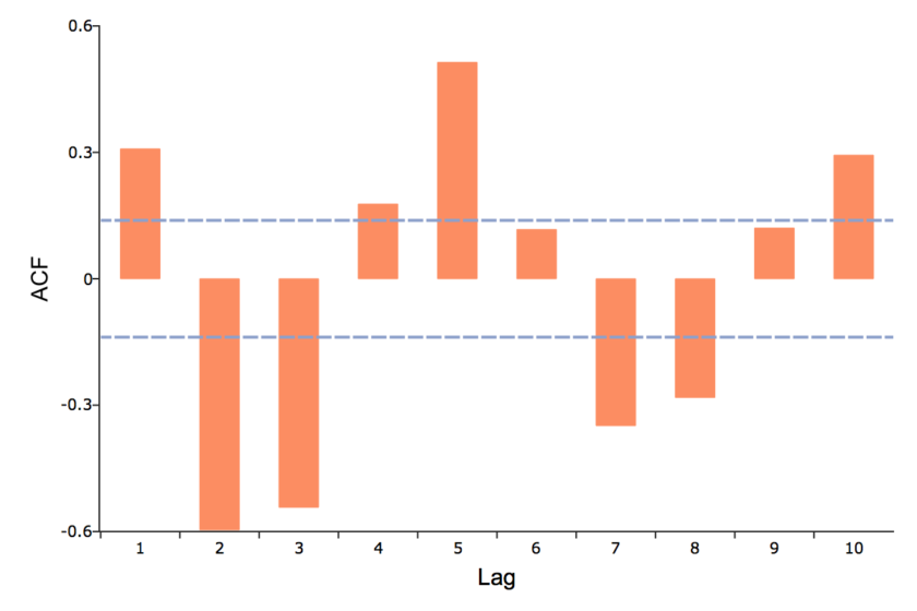
Plot the ACF
As an alternative to the printed table, a bar graph visually presents the autocorrelation information. The ACF can be computed and graphed using the GAUSS function plotACF. The plotACF function takes the same inputs as the acf function:
// Maximum number of autocorrelations
 k = 10;

// Order of differencing
 d = 0;

// Compute and plot the sample autocorrelations
 plotACF(y_sim, k, d);
The above code will produce a graph similar to the following:

© 2026 Aptech Systems, Inc. All rights reserved.
PARTIAL AUTOCORRELATIONS
The previous example is easily extended to find the PACF for the same randomly generated data.
The pacf function requires the following three inputs:
y
N x 1 data matrix.
k
Scalar denoting the maximum number of autocorrelations to compute. 0 < k < N.
d
Scalar denoting the order of differencing. If only computing the autocorrelations from the original time series, then d equals 0.
Compute the PACF
The example below will compute the partial autocorrelations for lags 1 through 10. It uses the y_sim variable created in the tutorial simulating ARIMA models.
 // Maximum number of autocorrelations
 k = 10;

// Order of differencing
 d = 0;

// Compute the partial autocorrelations
 p = pacf(y_sim, k, d);

// Display autocorrelations
 a_lab = seqa(1, 1, rows(p));
 print "Lags"$~"PACF";
 print ntos(a_lab~p, 4);
The above code produces the following output:
Lags PACF

1 0.3084
 2 -0.7639
 3 0.04611
 4 0.0185
 5 0.01686
 6 -0.0424
 7 -0.007356
 8 -0.03321
 9 -0.01139
 10 0.01927
Plot the PACF
The PACF can be computed and graphed using the GAUSS function plotPACF. The plotPACF function takes the same inputs as the pacf function:
 // Maximum number of autocorrelations
 k = 10;

// Order of differencing
 d = 0;

// Compute and plot the partial autocorrelation function
 plotPACF(y_sim, k, d);
CONCLUSION
You have learned how to compute and plot the ACF and PACF in GAUSS.